The annual bundle is named “Physics Papers 2018”, but the cover dates this ordinary-sitting paper to 13 June 2019. The year follows the cover. All eleven questions are solved, including all four choices in Section B and the separate introductory request in Question 11.
The successive derivatives are , so . Substitution in the Taylor series formula about givesThe ratio test shows convergence for every finite real or complex : the absolute ratio of successive terms is . This is also the usual exponential function series applied to , proving that the series equals the stated function everywhere.
The solid angle is the intercepted surface area on a sphere of radius , divided by . Take the cone axis as the polar axis of spherical coordinates, and call its half-opening angle . With polar integration variable ,For small measured in radians, the Taylor series of the cosine givesThis is the solid angle of a circular cone, measured in steradians.
The supplied angular diameter is twice the half-opening angle, soHence either apparent disc subtendsThe fraction is about of the entire celestial sphere. Using the angular diameter directly in would give four times the correct small-angle answer.
The real logarithm restricts the domain to . Differentiating givesSince cannot vanish in the domain, a stationary point requires . The logarithm is strictly increasing, so this equation has exactly one solution:The second derivative is , giving . In fact is negative below and positive above it, so the point is the unique global minimum on . The boundary value is not an additional stationary point, since the original function is not defined there.
For a continuous random variable with probability density function , its cumulative distribution function isConsequently wherever the density is continuous, and almost everywhere for an absolutely continuous distribution.
Here . Thus for . For , the event is . Symmetry of the Laplace distribution givesTherefore the square of a standard Laplace variable has cumulative distribution functionIt is continuous at zero, so there is no point mass there. As a check, its probability density function for is , whose integral becomes after setting .
Set . The chain rule gives , whileThusThe real domain excludes zero because the original denominator vanishes there; for it is strictly positive.
Take the normal vector to point outward from the box. The divergence theorem changes the closed-surface flux into a volume integral. The divergence isThe first term integrates to zero in , since . ThereforeHenceA direct face check gives zero from the two faces, from the pair of faces, and from the pair of faces. This also checks the outward-orientation signs.
Work in the small-slope model of a transverse wave on a taut string. Let be the constant tension, the linear mass density, and take a right-moving sinusoidal displacement , with wave number . The energy flux of a transverse string wave through a cut is the transverse force times transverse velocity:A cycle average gives . Using , obtained from the string wave equation, yieldsThe sign in the flux formula makes the power positive for propagation in the positive direction.
The energy per unit equilibrium length is the sum of the kinetic and elastic terms:For a segment of mass containing many wavelengths, the spatial average agrees with the cycle average up to a small endpoint correction. Thus . Convert the given quantities to SI units: , , and . ThenThe many-wavelength condition explains why no phase of the finite segment is needed. The result is exact as a cycle average, or for a segment containing an integer number of wavelengths.
Let the angular velocity vector be the spatially constant . Choose an origin on the fixed rotation axis. The velocity field of a rigid body is . In components,Taking the curl givesAn added spatially uniform translational velocity has zero curl, so it does not affect this relation. Equivalently, the vorticity of rigid rotation is twice the angular velocity; the local rotational part of a general smooth flow has angular velocity .
For an oriented piecewise smooth surface with boundary , and a vector field continuously differentiable on a neighborhood of , Stokes theorem statesHere is the chosen unit normal vector, is the unsigned surface area element, and is the tangent displacement along the boundary. The right-hand rule pairs the boundary orientation with . If there are several boundary components, the line integral includes all of them with their induced orientations.
A simply connected surface is connected and every closed loop on it can be continuously contracted to a point while remaining on the surface. A disc is an example. An annulus is not simply connected: a loop winding once around its hole cannot contract within it.
Stokes' theorem is valid for both types of surface, under the smoothness and orientation hypotheses above. Simple connectivity is not a requirement of the theorem. For a concrete annular example, take and in the horizontal plane. Its curl is , so the left side is . The right side is the counterclockwise outer-circle integral minus the counterclockwise inner-circle integral , giving exactly the same answer. Omitting the inner boundary would be an incorrect application of the theorem.
Write and work away from the axis, where . The vector field is independent of and has zero vertical component, so only the vertical curl can be nonzero:ThereforeThis local spin in an azimuthal power-law flow depends on the radial variation of the tangential speed, not merely on the sign of that speed.
In cylindrical coordinates, . The tangential coefficient is positive for every real and , so the large-scale circulation is always counterclockwise when viewed from positive .
By solution, the infinitesimal local angular velocity is . Its sign gives“Zero local spin” does not mean zero velocity: at a marked small element is still carried around the axis while its infinitesimal rotational component is zero. Orbital motion around the axis and local vorticity are different measurements.
For , the azimuthal unit vector is , soOn a counterclockwise circle at fixed height, . Henceindependent of the positive radius. Clockwise orientation reverses the sign.
There is no contradiction with the zero curl found in solution. The vector field is undefined on the axis, so it is not continuously differentiable on a disc spanning ; the hypotheses of Stokes theorem fail for that disc. It is smooth on a planar annulus excluding the axis, where Stokes theorem correctly gives zero: the two boundary line integrals cancel, .
The same check works for general . A counterclockwise circle has circulation . Integrating the curl over an annulus gives, for ,For , both sides are zero. Thus all three preceding results are consistent with Stokes theorem; the necessary distinctions are the regularity of the vector field and inclusion of every oriented boundary component.
Assume small transverse slopes, a flexible string, constant tension and uniform linear mass density . For an element of equilibrium length , the vertical force is the difference of the vertical tension components at its ends. To first order in slope,Its mass is and its transverse acceleration is . Newton's second law therefore gives , orThis is the one-dimensional wave equation for small-amplitude transverse waves. Changes in string length and horizontal acceleration are second order in slope and are neglected in this linear approximation.
At distance below the support, the cable must carry the weight of the remaining length . Thus its equilibrium tension is , and the local transverse wave speed isThe linear mass density cancels. More precisely the small-displacement equation with variable tension is ; its local characteristic speed is the expression above, even though a first-spatial-derivative term is also present.
The wave travel time on a hanging uniform cable is obtained from :Although the local speed tends to zero at the free end, the endpoint singularity in the travel-time integral is integrable. This finite result belongs to the ideal flexible-cable model, with bending stiffness neglected.
A dispersive medium has frequency-dependent phase velocity, so different Fourier components generally propagate with different phases. A dispersion relation specifies as a function of the wave number , or an equivalent relation between them. For a monochromatic factor , a point of fixed phase moves atFor a narrow wave packet centered at , expand . The envelope then translates at the group velocityThe phase velocity tracks crests of a monochromatic wave. The group velocity tracks a slowly varying envelope when the narrow-band approximation is valid; in the ideal lossless guide here it also equals the longitudinal energy-transport speed. It is not a universal formula for signal-front speed in every possible dispersive medium.
For the propagating branch of the supplied electromagnetic waveguide relation, take , and . Differentiation givesThe product alone would also allow ; the strictly positive cutoff is what makes the inequalities strict. At the phase-speed expression is undefined, and these formulas are interpreted through the propagating limit.
A moving monochromatic crest does not carry a new message. An information-bearing modulation is made from a range of frequencies; here its packet and energy move below , and the high-frequency limit approaches . Causal propagation of a newly switched-on disturbance is governed by the electromagnetic equations, so the superluminal phase velocity does not permit faster-than-light signalling. These are the waveguide phase and group velocities for a mode with nonzero cutoff, rather than a zero-cutoff mode with both velocities equal to .
Use for cylindrical radius, to distinguish it from spherical radius . In cylindrical coordinates , the azimuthal angle is measured from positive in the horizontal plane:Here and .
In spherical polar coordinates , take as the polar angle from positive and use the same azimuthal angle :The ranges are , and . The radial direction has horizontal projection of length , which explains the extra factor in . The azimuth is undefined on the polar axis, and both angles are nonunique at the origin; these are coordinate degeneracies rather than geometric singularities.
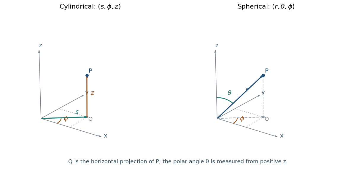

On the unit upper hemisphere, use spherical coordinates with and . The surface mass density is , while the surface area element is . Thus the total mass isThe answer is in the mass units implicit in the specified unit radius and density law. A useful geometric check is that on the unit hemisphere equals the area element of its vertical projection onto the horizontal unit disc, whose area is .
This is a scalar surface integral, not an oriented flux. Split the whole closed surface into the bottom disc, curved side and tilted top; shared edge curves have zero surface area.
On the bottom, and the integrand is . Its integral over the symmetric disc vanishes by oddness:On the top, , so . The graph has , , giving . HenceFor the side, let and parametrize by , with . The surface area element is . ThusAdding all three pieces givesThe tilted top remains above the bottom everywhere because . The calculation is an instance of a scalar surface integral over a cylinder with one tilted cap; reversing a surface orientation would not change any of its terms.
A normal mode is a motion of a linear oscillatory system in which every coordinate has the same angular frequency and a fixed relative amplitude and phase. For a conservative small-displacement system it has the formwhere is the mode shape, the stiffness matrix, and the mass matrix. Superposing normal modes gives the general small-oscillation motion when their eigenvectors form a complete basis.
Two common examples are standing transverse oscillations of a string fixed at both ends, and oscillations of coupled masses and springs. The string's mode shapes are sinusoidal along its length; the coupled system's mode shapes are fixed patterns of particle displacements. The following parts determine those patterns for the three-mass system in the source figure.
Let be longitudinal displacements from equilibrium, with positive direction to the right. The fixed walls have zero displacement. The first mass feels forces and ; the central mass feels and ; the last mass feels and . Hooke's law and Newton's second law therefore giveEquivalently,All four springs contribute: the wall springs supply one of the two diagonal terms in the first and third rows. This is a fixed-end chain, not a freely ended chain with a zero-frequency translation mode.
Put in solution. The normal mode equation is , with . Its characteristic polynomial isThe three eigenvalues are , , and . Solving the corresponding linear equations yieldsEach mode shape may be multiplied by any nonzero scalar. Their squared Euclidean norms are , respectively, so unit-normalized eigenvectors are . They are mutually orthogonal, as expected for the real symmetric stiffness matrix with equal masses.
The entries in the table are angular frequencies; the corresponding ordinary frequencies in cycles per unit time are . All three are positive because the fixed walls remove uniform translation as a free motion.
To specify “initial motion” unambiguously, choose each mode to pass through equilibrium at with proportional to its listed mode shape. The arrows in the figure then describe relative initial velocities:
- In mode 1, all three masses move in the same direction; the central mass has times either outer velocity.
- In mode 2, the two outer masses move with equal and opposite velocities, while the central mass remains stationary.
- In mode 3, the outer masses move together while the central mass moves oppositely with times their speed.
Reversing every arrow changes only the common phase. A quarter-cycle later these same ratios describe the extremal displacements, with zero instantaneous velocity.
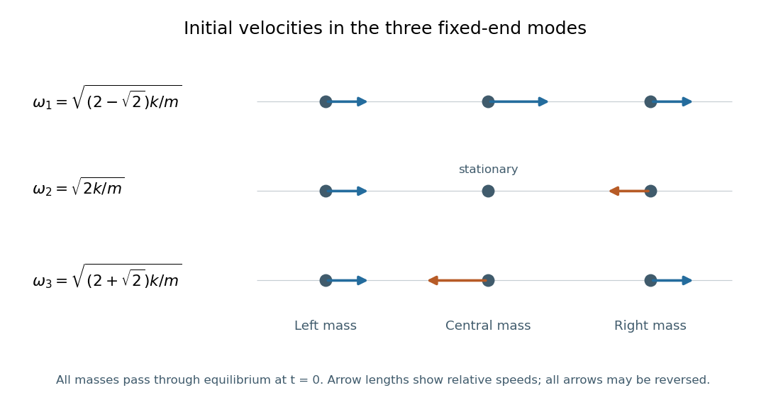
Relative initial velocities of the three fixed-end normal modes, starting as the masses pass through equilibrium.
Arrow lengths follow the mode shapes. The antisymmetric mode has equal and opposite outer velocities and zero central velocity; its angular frequency is unchanged by any positive change in central mass. Details.
Now replace the central mass by , leaving the outer masses equal to . The antisymmetric mode shape gives zero net force on the central mass, since . Each outer mass still obeys . ConsequentlyThis middle-mass-independent mode of a fixed three-mass spring chain is exact, not merely a large- approximation. The other two modes move the central mass and generally change. For example, their symmetric-sector frequencies satisfywhich explicitly depends on .
Articles by others on the same topic
There are currently no matching articles.