Past exam of the mathematics course of the University of Cambridge / 2010 / iii / Paper 28 (Advanced Probability)

Assume $0<p<1$, so the ratio defining $Z_n$ is meaningful. Extend the random walk by $S_0=0$, the filtration by a trivial ${\mathcal{F}}_0$, and the process by $Z_0=1$. Write $r=q/p$. Each $Z_n=r^{S_n}$ is ${\mathcal{F}}_n$-measurable and integrable, since $|S_n|\le n$. The next increment is independent of ${\mathcal{F}}_n$, soTherefore $\boxed{(Z_n{)}_{n\ge 0}\text{ is a nonnegative martingale},\mathbb{E}{Z}_n=1}$. This is the exponential martingale of a biased simple random walk, with exponent $\log (q/p)$. At $p=q=1/2$, it is the constant process one. The endpoint cases $p=0$ or $p=1$ require separate definitions and are not covered by the printed ratio.

The Doob maximal inequality for a nonnegative submartingale states that, for a nonnegative submartingale $(M_j{)}_{0\le j\le N}$ and $u>0$,For completeness, partition the crossing event according to its first crossing time $j$. On that event $M_j\ge u$, while $\mathbb{E}[M_N\mid {\mathcal{F}}_j]\ge M_j$. Summing the corresponding expectations over $j$ proves $u\mathbb{P}(\max M_j\ge u)\le \mathbb{E}[M_N{1}_{\{\max M_j\ge u\}}]\le \mathbb{E}{M}_N$.

If $q>p$, the exponential $r^{S_j}$, with $r=q/p>1$, is increasing as a function of $S_j$. Apply the inequality to the martingale from part (a), with $u=r^k$:Letting $N\to \infty$ and using continuity of probability measures on increasing events givesThe same event is obtained if the supremum excludes time zero, since $k\ge 1$. If $p\ge q$, the right side is at least one and the bound is automatic; the nontrivial Doob maximal inequality argument is for $q>p$.

For $q>p$, let $M={\sup }_{n\ge 0}{S}_n$, including $S_0=0$. It is a nonnegative integer-valued random variable, possibly infinite before the following estimate. The tail-sum formula for expectation and part (i) giveThus $\boxed{\mathbb{E}\underset{n\ge 0}{\sup }{S}_n\le p/(q-p)}$, and the supremum is finite almost surely. The sum identity follows by writing $M={\sum }_{k\ge 1}{1}_{\{M\ge k\}}$ and applying monotone convergence theorem. If the printed supremum is read literally over $n\ge 1$, its positive part has exactly the same positive-level tails and its negative part is bounded by one. The same upper bound on its expected value remains valid.

The increments have expected value $p-q<0$. The strong law of large numbers for independent and identically distributed random variables with finite absolute mean givesHence $S_n\to -\infty$. Since $q/p>1$,Its expected value nevertheless stays equal to one. Thus this martingale is not uniformly integrable, and it does not converge to zero in $L^1$. This distinction will be avoided in part (ii) by stopping at an upper level, which makes the stopped process bounded.

Let $r=q/p>1$ and $H_k$ be the first hitting time of level $k$. Nearest-neighbour steps imply $S_{H_k}=k$ whenever $H_k<\infty$: the walk cannot overshoot its first upward crossing. On this event the stopped martingale eventually has the constant value $r^k$. On $\{H_k=\infty \}$, it is $Z_n$ and tends to zero by part (i). ThereforeFor every $n$, $0\le Z_{n\wedge H_k}\le r^k$. Before the hit the walk is below $k$, and at the hit it equals $k$. The optional stopping theorem for the bounded stopping time $n\wedge H_k$ gives $\mathbb{E}{Z}_{n\wedge H_k}=\mathbb{E}{Z}_0=1$. The dominated convergence theorem now yields $1=r^k\mathbb{P}(H_k<\infty )$. ConsequentlyThe uniform bound on the stopped variables justifies the limit; applying optional stopping directly at the possibly infinite $H_k$ without this argument would not be valid.

Put $\rho =p/q\in (0,1)$ and $M={\sup }_{n\ge 0}{S}_n$. For $k\ge 1$, $\{M\ge k\}=\{H_k<\infty \}$, so part (ii) gives $\mathbb{P}(M\ge k)={\rho }^k$. Since $\mathbb{P}(M\ge 0)=1$, taking differences givesThis is the geometric distribution of parameter $1-p/q$ on the failures-before-first-success convention, with support $\{0,1,\dots \}$. Its expected value is $\rho /(1-\rho )=p/(q-p)$, so the bound in part (b)(ii) is attained. This proves the maximum of a downward-biased random walk formula.

The time-zero convention is necessary here. If $M_1={\sup }_{n\ge 1}{S}_n$, then the first step can be $-1$ and the walk may never return to zero. Using the same hitting probability calculation after that step gives $\mathbb{P}(M_1=-1)=q(1-\rho )=q-p>0$. Also $\mathbb{P}(M_1\ge 0)=p+q\rho =2p$, while its tails at positive $k$ remain ${\rho }^k$. Its masses are thereforeThus the printed geometric conclusion is correct for the standard maximum that includes $S_0=0$, and false for a supremum restricted to the positive times.

For each fixed $t\in [0,1]$, the variables $1_{\{X_k\le t\}}$ are independent and identically distributed random variables with Bernoulli distribution of parameter $t$. Their expected value is $t$, and the strong law of large numbers gives $F_n(t)\to t$ almost surely.

For a finite set $F$, intersect these probability-one events over its finitely many elements. On the resulting single event, every one of the finitely many errors tends to zero, so their maximum tends to zero:If $F$ is empty, take the displayed maximum to be zero. The important point is simultaneous convergence on one event; pointwise convergence at an uncountable collection of arguments would not alone imply the uniform claim in part (ii).

For each positive integer $m$, apply part (i) to the grid $D_m=\{j/m:0\le j\le m\}$. Intersect the resulting probability-one events over all $m$, a countable intersection. Work on this common event.

For $x\in [j/m,(j+1)/m]$, monotonicity of the empirical distribution function gives $F_n(j/m)\le F_n(x)\le F_n((j+1)/m)$. ConsequentlyandThe endpoint $x=1$ is itself on the grid. ThereforeFor each fixed $m$, take the upper limit as $n\to \infty$; part (i) makes the maximum vanish. Then let $m\to \infty$. This provesThis is the uniform-sample case of the Glivenko-Cantelli theorem, proved by a finite-grid approximation rather than assumed.

Let $G$ be the cumulative distribution function of the arbitrary Borel probability measure $\mu$. It may have atoms or flat intervals. Use its quantile functionThe limits of $G$ at the two infinities make $Q(u)$ finite. Its monotonicity and right continuity imply the exact equivalence $Q(u)\le x⟺u\le G(x)$. For the nontrivial direction, if $Q(u)\le x$, points with $G\ge u$ lie arbitrarily close above $Q(u)$; if the infimum itself is $x$, right continuity gives $G(x)\ge u$. The other direction follows directly from the defining infimum.

Take independent uniform variables $U_k$ and set $Y_k^{\prime }=Q(U_k)$. Thenso $(Y_k^{\prime })$ has the same entire sequence law as the original iid sample $(Y_k)$. On this construction, the empirical distribution function satisfiesThus part (ii) givesThe supremum is measurable: since both distribution functions are right-continuous, it equals the supremum over rational $x$. The convergence event consequently depends measurably on the coordinate sequence, and equality of the sequence laws transfers its probability one to $(Y_k)$. HenceThis is the Quantile proof of the Glivenko-Cantelli theorem, including arbitrary distributions with atoms. The original PDF supplies the full definition and absolute-value signs in this part, which the TeX conversion incompletely records.

A real Gaussian process $(Z_t{)}_{t\in T}$ is a family of random variables such that every finite vector $(Z_{t_1},\dots ,Z_{t_d})$ has a multivariate normal distribution, allowing degenerate distributions. Equivalently every finite real linear combination is a Gaussian random variable. Its mean and covariance kernel are $m(t)=\mathbb{E}{Z}_t$ and $C(s,t)=\mathbb{E}[(Z_s-m(s))(Z_t-m(t))]$.

For any finite set of indices, these functions give the whole mean vector and covariance matrix. The characteristic function of the vector isThe standard uniqueness theorem for characteristic functions therefore determines every finite-dimensional distribution, including the singular cases. Cylinder events form a generating class for the product sigma-algebra on ${\mathbb{R}}^T$ and are closed under finite intersections, so agreement on all cylinder events gives agreement of the process laws by the uniqueness theorem for probability measures. Thus the mean and covariance determine the law on this coordinate sigma-algebra even when $T$ is uncountable. This statement does not claim uniqueness on an arbitrary finer sigma-algebra of path properties.

Let $(B_t{)}_{0\le t\le 1}$ be standard Brownian motion with its continuous version, and defineEvery finite vector is a linear transform of a Gaussian Brownian vector, so $Z$ is a centred Gaussian process. Using $\mathbb{E}[B_s{B}_t]=\min (s,t)$,For $s\le t$, this is $s(1-t)$, the prescribed Brownian bridge covariance kernel. Its paths are continuous on the probability-one event of Brownian continuity, because $t\mapsto t{B}_1$ is continuous on every sample. The construction also gives $Z_0=Z_1=0$. Thus it realizes a Brownian bridge with almost surely continuous paths, and part (i) identifies its process law.

Fix times $t_1,\dots ,t_d\in [0,1]$, and setThese are iid bounded centred random vectors, andTheir covariance matrix isWe prove the required central limit theorem calculation explicitly. For $u\in {\mathbb{R}}^d$, the scalar $u\cdot V_1$ is bounded, has mean zero and second moment $u^{T}Cu$. The Taylor expansion of the exponential, with its uniformly bounded cubic remainder, givesIndependence implies that the characteristic function of the sum vector is the $n$th power of this expression, so it tends to $\exp (-u^{T}Cu/2)$. This is the characteristic function of a centred multivariate normal distribution with covariance $C$. The Lévy continuity theorem states that convergence of characteristic functions to a characteristic function continuous at zero gives convergence in distribution; apply it here.

By part (ii), the corresponding Brownian bridge vector has exactly this covariance and mean. ThereforeRepeated times or the endpoint times may make $C$ singular; the characteristic-function argument still applies. This proves every finite-dimensional distribution convergence requested, the uniform case of the Finite-dimensional Brownian bridge limit of an empirical distribution process.

Here $F=1_A$ is bounded and hence lies in $L^2$ as well as $L^1$. Conditional expectation on a sub-sigma-algebra is the orthogonal projection in $L^2$ onto its measurable subspace. We can use these projections to justify both limits without any symmetry assumption on the probability measure.

The increasing coordinate sigma-algebras ${\mathcal{E}}_n$ generate the whole product sigma-algebra $\mathcal{F}$. Functions depending on finitely many coordinates are dense in $L^2(\mathcal{F})$: their cylinder indicators generate $\mathcal{F}$, and the usual monotone-class approximation proves density of their linear span. If a cylinder function $V$ is ${\mathcal{E}}_N$-measurable, then for $n\ge N$ the $L^2$ projection contraction givesApproximate $F$ arbitrarily well by such $V$ to prove the first $L^2$ limit.

For the decreasing tail sigma-algebras ${\mathcal{G}}_n$, put $Y_n=\mathbb{E}[F\mid {\mathcal{G}}_n]$. If $m\ge n$, the tower property gives $\mathbb{E}[Y_n\mid {\mathcal{G}}_m]=Y_m$. Projection orthogonality therefore yieldsThe norms on the right decrease and are nonnegative, so $(Y_n)$ is Cauchy in $L^2$ and has a limit $Y$. Choose an almost-surely convergent subsequence and take its pointwise upper limit. For every fixed $n$ its tail consists of ${\mathcal{G}}_n$-measurable functions, so this supplies a version of $Y$ measurable with respect to every ${\mathcal{G}}_n$, hence to $\mathcal{G}={\bigcap }_n{\mathcal{G}}_n$. For any $C\in \mathcal{G}$, $\mathbb{E}[Y_n{1}_C]=\mathbb{E}[F{1}_C]$; passing to the limit identifies $Y=\mathbb{E}[F\mid \mathcal{G}]$.

Finally $\Vert W{\Vert }_1\le \Vert W{\Vert }_2$ on a probability space, by the Cauchy-Schwarz inequality. ThusThese are the increasing-filtration and reverse martingale convergence theorem limits; the argument above establishes the requested norm convergence directly.

Let $T$ swap coordinate blocks $0,\dots ,n$ and $n+1,\dots ,2n+1$, fixing all other coordinates. The symmetric law makes $T$ measure preserving, and invariance of the event $A$ gives $F\circ T=F$ pointwise. Put ${\mathcal{B}}_n=\sigma (X_{n+1},\dots ,X_{2n+1})$.

Conditional expectation transforms covariantly under this block swap:To check it, the left side is ${\mathcal{B}}_n$-measurable, and for $C\in {\mathcal{B}}_n$ the change of variables by $T$ sends its defining integral to the conditional-expectation identity on $T(C)\in {\mathcal{E}}_n$, with $F\circ T=F$. Thus the two versions agree. Measure preservation now givesThis is the first requested estimate.

The L1 contraction of conditional expectation follows from the pointwise bound $|\mathbb{E}[Z\mid \mathcal{H}]|\le \mathbb{E}[|Z|\mid \mathcal{H}]$: take expectations to get $\Vert \mathbb{E}[Z\mid \mathcal{H}]{\Vert }_1\le \Vert Z{\Vert }_1$. Applied to a difference, it makes conditional expectation a contraction between any two integrable inputs.

Let $U_n=\mathbb{E}[F\mid {\mathcal{B}}_n]$. Since ${\mathcal{B}}_n\subseteq {\mathcal{G}}_n$, $U_n$ is ${\mathcal{G}}_n$-measurable. HenceCombining this with the other given approximation bound yieldsThe left side does not depend on $n$, and $\epsilon >0$ was arbitrary. It is therefore zero. For a $\mathcal{G}$-measurable version $Y=\mathbb{E}[F\mid \mathcal{G}]$, the event $C=\{Y>1/2\}$ belongs to $\mathcal{G}$ and satisfiesThis proves that exchangeable invariant events are tail events modulo null sets. It does not assert literal pointwise equality of the two events or sigma-algebras before completing them with null sets.

Let $T_{\pi }$ permute coordinates $0,\dots ,m$, fixing the later coordinates. For any integrable random variable $V$, its group averageis invariant under this group, hence ${\mathcal{S}}_m$-measurable. If $C\in {\mathcal{S}}_m$, invariance of $C$ and measure preservation of each $T_{\pi }$ give $\mathbb{E}[1_{C}V\circ T_{\pi }]=\mathbb{E}[1_{C}V]$. Thus $A_{m}V$ satisfies the integral definition of $\mathbb{E}[V\mid {\mathcal{S}}_m]$. This proves symmetrization as conditional expectation.

Apply it to $V=1_{A_k}(X_k)$ for $m\ge k$. Under a uniform permutation of $m+1$ coordinates, its selected coordinate is uniform among all of them, soThe reverse martingale convergence theorem says that, for decreasing sigma-algebras ${\mathcal{H}}_m$ and an integrable $V$, these conditional expectations converge almost surely and in $L^1$ to $\mathbb{E}[V\mid {\bigcap }_m{\mathcal{H}}_m]$. Here ${\mathcal{S}}_m\downarrow \mathcal{S}$, because every finitely supported permutation belongs to one of the finite groups. ThereforeIntersect these probability-one events for the finitely many $k=0,\dots ,p$ and multiply the limits. Expanding the product of finite sums givesThe sum here includes repeated indices. No independence of the original coordinates was assumed; exchangeability and reverse conditional-expectation convergence are precisely what replaced it.

Put $N=m+1$ and $d=p+1$. Average $V={\prod }_{k=0}^p{1}_{A_k}(X_k)$ over all permutations of the first $N$ coordinates, as justified in part (a). For any prescribed ordered tuple of $d$ distinct images $({\ell }_0,\dots ,{\ell }_p)$, exactly $(N-d)!=(m-p)!$ permutations produce that tuple. ThereforeThe denominator is the falling factorial $(N{)}_d=N!/(N-d)!$, with exactly $p+1$ factors. The sum must be over ordered distinct tuples: its $k$th coordinate is attached to $A_k$, and these sets need not be equal. This is the finite-sample version of symmetrization as conditional expectation.

The original PDF, as well as the TeX, prints the final factor as $m+1-p+1$. That is an off-by-one error: it must be $m+1-p$. With every $A_k=\mathbb{R}$, the conditional expectation is one and the numerator counts exactly $(N{)}_d$ ordered distinct tuples. This forces the normalization above and immediately detects the printed error. Interpreting the sum as unordered subsets would likewise give the wrong normalization and would lose the assignments to the different $A_k$.

Let $U_m$ be the average over all $d=p+1$ coordinate tuples in part (a), and $V_m$ the distinct-tuple average in part (b). Every product summand lies in $[0,1]$. A proportion ${\alpha }_m=(N{)}_d/N^d$, where $N=m+1$, of all tuples have distinct coordinates. Thuswhere $W_m\in [0,1]$ is the average over the remaining tuples. If there are no remaining tuples, the error is zero. Hence $|U_m-V_m|\le 1-{\alpha }_m$.

For $d$ independent uniform choices from $N$ indices, any particular pair coincides with probability $1/N$. A union bound over the $\left(\genfrac{}{}{0ex}{}{d}{2}\right)$ pairs givesThis deterministic sampling with and without replacement comparison for bounded products is the needed link between the two averages.

Part (a) identifies the almost-sure limit of $U_m$ as ${\prod }_{k=0}^p\mathbb{E}[1_{A_k}(X_k)\mid \mathcal{S}]$. By part (b) and the reverse martingale convergence theorem, $V_m$ converges almost surely to $\mathbb{E}[{\prod }_{k=0}^p{1}_{A_k}(X_k)\mid \mathcal{S}]$. Their difference vanishes, soThis is precisely conditional independence. Exchangeability also makes the single-coordinate conditional laws identical, by applying a coordinate transposition and testing against invariant events. The result is the De Finetti theorem, established here by finite symmetrization and the vanishing collision fraction.

Write $f=u+iv$. The prescribed complex-linear differential is exactly the Cauchy-Riemann equationsA holomorphic function is smooth, as follows locally from its Cauchy integral formula, so its mixed second partial derivatives commute. Differentiating the two equations givesand, rewriting them as $v_x=-u_y$, $v_y=u_x$,Thus $\boxed{\Delta \Re f=\Delta \Im f=0}$: both components are harmonic functions. Here $\Delta ={\partial }_x^2+{\partial }_y^2$, the sign convention used for the Brownian generator $\Delta /2$.

Let $u=\Re f$, and suppose $u$ has a local maximum at $z_0\in U$. Choose $R>0$ such that the closed disk $\overline{D(z_0,R)}$ lies in $U$ and $u(z)\le u(z_0)$ throughout it. Start planar Brownian motion $B$ at $z_0$, and for $0<r<R$ let ${\tau }_r$ be its first exit from $D(z_0,r)$.

By part (a) and Itô formula, $u(B_{t\wedge {\tau }_r})$ is a local martingale; boundedness of $u$ on the compact disk makes it a true bounded martingale. The exit time is finite almost surely. One direct check applies the same formula to $|B_{t\wedge {\tau }_r}-z_0{|}^2$, giving $2\mathbb{E}(t\wedge {\tau }_r)=\mathbb{E}|B_{t\wedge {\tau }_r}-z_0{|}^2\le r^2$. Thus $\mathbb{E}{\tau }_r\le r^2/2$.

The optional stopping theorem, first at $t\wedge {\tau }_r$ and then by bounded convergence, givesThe exit point is uniformly distributed on the circle: rotational invariance of planar Brownian motion about its starting point makes its exit law rotation invariant, and normalized arc length is the unique rotation-invariant probability measure on a circle. Since every boundary value is at most $u(z_0)$, equality of the mean forces every boundary value to equal $u(z_0)$; continuity rules out a strict deficit at any boundary point. This holds for every $0<r<R$, so $u$ is constant on the entire disk.

The Cauchy-Riemann equations then give both partial derivatives of $v=\Im f$ equal to zero there. Thus $f$ is constant on that disk. The identity theorem for holomorphic functions propagates this constant to the connected component of $z_0$ in $U$. Applying the same Brownian argument to $v$ proves the assertion for the imaginary part as well:If $U$ is connected, this is constancy on all of $U$. For a disconnected open set the printed global wording needs this qualification: a function taking different constants on two disjoint disks is holomorphic and has local maxima on each disk while not being globally constant.

Suppose $|g|$ has a local maximum at $z_0$. If $g(z_0)=0$, the nonnegativity of the modulus forces $g=0$ throughout a neighbourhood, and the identity theorem for holomorphic functions makes it zero on that connected component.

If $g(z_0)\ne 0$, take $c=2i/g(z_0)$. Then $cg(z_0)=2i$, and continuity gives a disk $D$ around $z_0$ on which $\Im (cg)>1$. This lies within the given half-plane for a branch of the holomorphic logarithm. On $D$ defineComposition preserves holomorphy, and the real logarithm is strictly increasing, so $\Re f$ has a local maximum at $z_0$. Part (i) forces $f$ to be constant on the disk. Exponentiating gives $cg=e^f$, hence $g$ is constant there and, by the identity theorem for holomorphic functions, on the whole connected component. ThereforeThis proves the maximum modulus principle by the requested logarithm argument. Multiplication by $c$ is what puts the image in the supplied logarithm branch; no global logarithm of $g$ is assumed.

Suppose a nonconstant polynomial $P$ has no zero in $\mathbb{C}$. Its reciprocal $g=1/P$ is then an entire holomorphic function. If $d\ge 1$ is the degree and $a_d\ne 0$ its leading coefficient, division by $z^d$ shows $P(z)/z^d\to a_d$ as $|z|\to \infty$. Hence $|P(z)|\to \infty$, so $g(z)\to 0$. Continuity on compact disks now makes $g$ bounded on all of $\mathbb{C}$.

Fix $z\in \mathbb{C}$ and let $B$ be standard planar Brownian motion started at zero. By part (a) and Itô formula, both components of $g(z+B_t)$ are local martingales. Since $g$ is bounded, they are true martingales, andFor $\epsilon >0$, choose $R$ such that $|g(w)|\le \epsilon$ whenever $|w|>R$, and write $K={\sup }_w|g(w)|$. The two-dimensional Gaussian density of $z+B_t$ is bounded by $1/(2\pi t)$, soConsequentlyLet $t\to \infty$, then $\epsilon \downarrow 0$, to obtain $g(z)=0$. This is impossible for $1/P$. ThusThis Brownian proof of the fundamental theorem of algebra uses only harmonicity, the bounded-martingale property and the spreading Gaussian transition density. It does not use either maximum principle from part (b), nor does it incorrectly assume that planar Brownian motion hits a specified point.

Again suppose $P$ is a nonconstant polynomial without a complex zero, and put $g=1/P$. As proved in part (c), $g$ is an entire holomorphic function with $|g(z)|\to 0$ at infinity. Choose $z_0$ and then a disk large enough that $|g(z)|<|g(z_0)|/2$ outside it. On the closed disk, $|g|$ attains its maximum by the extreme value theorem, and that maximum is positive and greater than every value outside the disk. It is therefore a global, and in particular local, maximum on $\mathbb{C}$.

Part (b)(ii) forces $g$ to be constant. A nonzero constant reciprocal makes $P$ constant, a contradiction. Hence $\boxed{P\text{ has a complex zero}}$. Equivalently one can minimize $|P|$ globally and apply the maximum modulus principle to its reciprocal if that minimum is positive. This supplies the second proof of the fundamental theorem of algebra using part (b).

Use standard Brownian motion, started at $X_0=0$. Fix $0\le \alpha <\beta$, and divide $[\alpha ,\beta ]$ into $N$ equal subintervals. Its Brownian increments are independent centred normal random variables with strictly positive variance, so each is nonnegative with probability $1/2$. A nondecreasing path on the entire interval must have every one of these increments nonnegative. Hencefor every $N$, and therefore this probability is zero.

There are only countably many pairs of rational endpoints $0\le \alpha <\beta$. Take the union of the corresponding null events. Every interval of positive length, even one selected depending on the path, contains an interval with rational endpoints. Outside that single null event no such interval can be nondecreasing. ThusApplying the same argument to $-X$ also rules out nonincreasing intervals, the full nowhere monotonicity of Brownian motion property.

For each deterministic $a>0$, the Brownian reflection principle givesso $H_a$ is finite almost surely; $H_0=0$. Here $\Phi$ is the standard normal cumulative distribution function. The same reflection formula at levels decreasing to zero gives $\mathbb{P}({\sup }_{s\le \epsilon }{X}_s\le 0)=0$ for every $\epsilon >0$. Taking a countable intersection over $\epsilon =1/n$ shows that Brownian motion exceeds zero arbitrarily soon after its start.

By the Strong Markov property at the finite stopping time $H_a$, the process $X_{H_a+t}-a$ is fresh standard Brownian motion. It therefore exceeds zero arbitrarily soon. Path continuity gives $S_a\ge H_a$, and the preceding fact gives the reverse inequality. ConsequentlyThe exceptional event may depend on $a$; this does not imply simultaneous equality for all levels.

To exhibit the difference, set $A={\max }_{0\le t\le 1}{X}_t$, a random level. The reflection formula gives $A>0$ almost surely. Also $A>X_1$ almost surely: if $X_1$ were the maximum, the reversed increment process $Y_s=X_1-X_{1-s}$ would be nonnegative throughout $[0,1]$. This process has the law of standard Brownian motion, whose probability of staying nonnegative from zero is zero by reflection and symmetry. The level $A$ is attained at some time strictly before one, so $H_A<1$. It is not exceeded by time one, and continuity with $X_1<A$ gives a further positive interval before it can be exceeded. ThusAll these passage times exist simultaneously on the probability-one event where the Brownian path is continuous and unbounded above, obtained by intersecting the finite-hitting events for positive integer levels.

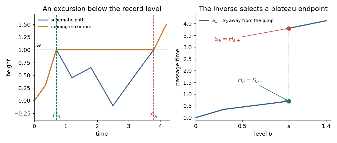
The illustration shows the pathwise mechanism. The Brownian running maximum stays flat during an excursion below an attained record. The non-strict inverse chooses the beginning of that plateau, while the strict generalized inverse of a nondecreasing function chooses its end. The curve is a schematic of this mechanism, not a claim of piecewise linear Brownian paths. The fixed-level equalities give the modification of a stochastic process relation, while the random-level discrepancy rules out indistinguishability of stochastic processes. This is fixed-level versus simultaneous Brownian passage-time equality.

Under the path convention used here, a real Lévy process $(L_a{)}_{a\ge 0}$ starts at zero, has independent increments and stationary increments, is stochastically continuous, and has càdlàg paths almost surely. We verify all four requirements for $S$.

The immediate positive excursions proved in part (b) give $S_0=0$. For a deterministic $a\ge 0$, $S_a$ is an almost-surely finite stopping time, and continuity gives $X_{S_a}=a$. The Strong Markov property implies that ${\tilde{X}}_t=X_{S_a+t}-a$ is a fresh Brownian motion independent of the information up to $S_a$. For $b\ge 0$,No crossing of $a+b$ could have occurred before $S_a$. The increment thus has the same law as $S_b$ and is independent of the past. Apply this successively at a finite increasing sequence of deterministic levels to prove stationary independent increments.

For $h>0$ and $\epsilon >0$, part (b) and reflection giveHence $S_h\to 0$ in probability. Stationarity of the increments gives stochastic continuity at every level, from either side where defined.

For path regularity, on a single probability-one event the Brownian running maximum $M_t={\max }_{s\le t}{X}_s$ is continuous, nondecreasing and unbounded, andThis inverse is nondecreasing. If $a_j\downarrow a$, then $S_{a_j}\downarrow L\ge S_a$. For any $t>S_a$, some $u<t$ has $M_u>a$; for all sufficiently large $j$, $M_u>a_j$, so $S_{a_j}\le u<t$. Thus $L=S_a$, proving right continuity at every level simultaneously. On each bounded level interval it is bounded by the finite value at a larger integer level. Monotonicity then gives finite left limits. ThereforeThe Brownian first-passage subordinator is the level-indexed increasing process, rather than a process indexed by the original Brownian time.