Past exam of the mathematics course of the year 1 of the natural sciences course of the University of Cambridge / 2014 / Paper 2

The $z$ component of the cross product is $2a-2$. For the result to lie in the $x$-$y$ plane, it must vanish, giving $a=1$. The dot product condition is then $2a+2-3b=0$, so

Using the exponential definition of the hyperbolic cosine and Euler's formula,Therefore

Multiply the standard Taylor series through quadratic order:The linear term is $x$ and the quadratic coefficient is $1-1/2$, hence

The characteristic equation of the homogeneous equation is $(r-1)(r-3)=0$. Thus the complementary function isA linear trial $y_p=ax+b$ gives $3ax+(3b-4a)=3x$, so $a=1$, $b=4/3$. One particular integral is therefore $\boxed{y_p=x+4/3}$.

Take the Cartesian partial derivatives component by component. The divergence isThe constant third component has zero derivatives. The curl consequently has only two nonzero components:

Set $\xi =x-ct$. The chain rule gives $u_t=-c{f}^{\prime }(\xi )$ and $u_x=f^{\prime }(\xi )$, so $u_t+c{u}_x=0$ for any differentiable $f$. The initial profile fixes $f(\xi )=\cos \xi$, givingThis is the translated initial profile, as described by the transport equation.

The vectors $(1,1)$ and $(1,-1)$ are eigenvectors, with respective eigenvalues $\cosh \varphi +\sinh \varphi$ and $\cosh \varphi -\sinh \varphi$. The exponential definitions reduce these toAt $\varphi =0$ they coincide and the matrix is the identity.

Stationarity requires both first partial derivatives to vanish:For example, choosing $x=\pi$ and $\cos y=0$ gives two points strictly inside the prescribed rectangle:Both satisfy the two derivative equations directly.

Only the $x$ component of the vector field is nonzero, so $\mathbf{F}\cdot d\mathbf{r}=(x^2+y^2)dx$. On the vertical segment, $dx=0$ throughout. Hence

On the horizontal segment $y=0$, while $x$ decreases from $1$ to $-1$. Keeping this orientation givesThe minus sign follows from traversing opposite to the positive $x$ direction.

The support is $x\ge 1$, and its normalized Pareto distribution density integrates to

Integrate the probability density function over the specified interval:The endpoint inclusions make no difference for this continuous distribution.

Let $C$ mean control-group membership and $E$ the adverse event. Equal allocation gives $P(C)=P(C^c)=1/2$, so the law of total probability gives $P(E)=(p_0+p_1)/2$. Bayes' theorem then givesThis is defined when $p_0+p_1>0$. If both are zero, the conditioning event has zero probability and the stated conditional probability is undefined.

Normalize the Rayleigh distribution by substituting $s=x^2/(2{\sigma }^2)$:For its sketch, the density starts at zero, is positive for $x>0$, and tends to zero at infinity. Differentiation givesIt therefore has a single maximum at $x=\sigma$, with height $e^{-1/2}/\sigma$.

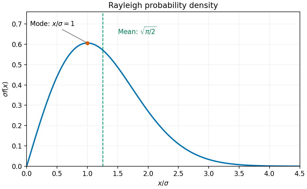
The expected value isIntegrating by parts with $xdx{e}^{-x^2/(2{\sigma }^2)}=-{\sigma }^{2}d(e^{-x^2/(2{\sigma }^2)})$ makes the boundary term vanish and leaves ${\int }_0^{\infty }{e}^{-x^2/(2{\sigma }^2)}dx$. The Gaussian integral gives

Use the usual model of independent games, each with Sheila-win probability $\theta$. After $m+n$ games, an outcome with $m$ wins and $n$ losses has $\left(\genfrac{}{}{0ex}{}{m+n}{m}\right)$ possible orders. Since both totals are below eleven, none of those sequences has already ended the match. ThusFor a completed Sheila win with $n$ losses, the last game must be her eleventh win. The preceding $10+n$ games contain ten wins and $n$ losses, so their probability is $\left(\genfrac{}{}{0ex}{}{10+n}{10}\right){\theta }^{10}(1-\theta {)}^n$, followed by one further factor $\theta$. The allowed loss counts are $0\le n\le 10$, and these terminal events are disjoint. HenceThis is the match win probability with a fixed winning score, obtained by the negative binomial stopping argument. Constant marginal game-win probabilities alone would not justify the product without the usual independence assumption.

A real square orthogonal matrix $Q$ satisfiesequivalently $Q^{-1}=Q^T$. Its columns, and also its rows, form an orthonormal basis. Consequently it preserves dot products and Euclidean norms.

To invert the matrix, row-reduce the augmented matrix $(M\mid I)$. Subtracting row one from rows two and three gives left rows $(0,-4,1)$ and $(0,0,2)$, so the pivots are nonzero and back-substitution is possible. The resulting matrix inverse isMultiplying by $M$ verifies the identity matrix. This inverse is not $M^T$; indeedThus $M$ is not orthogonal.

Use the order-reversal rule for the transpose of a product:Therefore the product of two orthogonal matrices is orthogonal. The argument does not require $A$ and $B$ to commute.

Collect the coefficients of the unknowns into the matrix and the constants into a column. The requested linear system isThe unknown coordinate $y$ here is a scalar component; the right-hand column is the vector denoted by the question's matrix-form notation.

At $a=2$, eliminate the first column by $R_2\leftarrow R_2-2R_1$ and $R_3\leftarrow R_3-2R_1$ in the augmented matrix. The last two rows give $-z=-2$ and $-y+z=-1$. Hence $z=2$, $y=3$, and the first row then gives $x=-2$. ThusThe coefficient determinant at this parameter is nonzero, so this solution is unique.

The same elimination at general $a$ gives the rowsThe coefficient determinant is $(a-3)(a-1)$. Only $a=1$ or $a=3$ can therefore fail to have a unique solution. At $a=3$, the second row reads $0=-2$, so there is no solution. At $a=1$, the last two rows are proportional and both specify $z=1$, leaving one free unknown; hence there are infinitely many solutions. Every other real $a$ gives a unique solution.

At $a=1$, the reduced system gives $z=1$ and $x+y=2$. Thus all solutions areGeometrically the solution set is an affine straight line, and substitution verifies all three original equations.

The hyperbolic identity ${\cosh }^{2}x-{\sinh }^{2}x=1$ and $\cosh x+\sinh x=e^x$ reduce the integrand to $1+e^x$. Therefore

Let $D=3x^2+2x+2$. Splitting the numerator into a derivative term and a constant gives $x-1=D^{\prime }/6-4/3$. ThusComplete the square as $D=((3x+1{)}^2+5)/3$ and substitute $u=3x+1$. The remaining integral is $\int du/(u^2+5)=\arctan (u/\sqrt{5})/\sqrt{5}$. HenceThe quadratic denominator is positive for all real $x$, so no logarithmic absolute value or real-domain exclusion is needed.

The argument $3x^3+2x$ is odd, so its squared sine is even. Replacing $x$ by $-x$ interchanges the numerator and denominator inside the logarithm, changing that factor's sign. Thus the full integrand is an odd function. It is continuous on the symmetric interval because $|x|\le 1/\pi <1$. Therefore

The fundamental theorem of calculus states that integrating a continuous function from a fixed lower endpoint produces an antiderivative. More precisely, if $f$ is continuous at the interior point $x$, thenIndeed, the difference quotient is the average of $f$ over the short interval from $x$ to $x+h$, which tends to $f(x)$ by continuity. The accompanying evaluation rule is ${\int }_a^{b}f=F(b)-F(a)$ whenever $F^{\prime }=f$ on the interval.

The sum is finite, so differentiation passes through it without a convergence issue. Each lower limit $n$ is constant with respect to $x$, and the fundamental theorem of calculus gives the same upper-end integrand. Hence the derivative isThe binomial theorem at $1+1$ gives the sum $2^N$. Therefore

Writing the two coefficients as $M,N$, their mixed derivatives satisfy $M_y=2xy=N_x$, so the smooth form is exact on ${\mathbb{R}}^2$. Integrating the first coefficient with respect to $x$ gives $f=2x^2+x^2{y}^2/2+h(y)$. Matching $f_y=y+x^{2}y$ gives $h^{\prime }(y)=y$. One potential is thereforeThe integral curves of $df=0$ are its level curves. Absorbing a factor of two into the constant giveson real graph branches. The initial condition fixes $C=12$ and selects the positive branch:This is the maximal smooth graph interval containing $x=1$; at either endpoint the level curve has a vertical tangent, so $y^{\prime }$ cannot remain finite.

Exactness after multiplication requires ${\partial }_y(\mu M)={\partial }_x(\mu N)$. Since $\mu$ depends only on $x$,For $\mu =\exp (\int f(x)dx)$, the ratio ${\mu }^{\prime }/\mu$ is $f(x)$, soThe assumed existence means this ratio is a function only of $x$ wherever the division is valid. For a factor depending only on $y$, the corresponding equation is ${\psi }^{\prime }M+\psi M_y=\psi N_x$, givingThese are the integrating factor for a differential one-form formulas. Nonzero constant multiples are equivalent. Exactness follows locally from closedness, and globally on a suitable simply connected domain.

Here $M_y-N_x=(6xy+2)-(4xy+1)=2xy+1$, whereas $N=x(2xy+1)$. Thus the ratio in (b) is $1/x$, and one may choose the nonzero integrating factor $\boxed{\mu (x)=x}$ on either half-line. A negative constant multiple on a half-line is harmless.

The multiplied form isHence $x^3{y}^2+x^{2}y=C$, a quadratic equation for $y$. Solving it givesChoose a real branch with positive discriminant to obtain a differentiable graph; a zero discriminant produces a vertical tangent. Although the ratio derivation initially cancels $2xy+1$, the displayed exact differential verifies the multiplying factor directly wherever $x\ne 0$. At $C=0$ the branches are $y=0$ and $y=-1/x$. Only $y=0$ has a finite smooth extension across $x=0$, where the original equation requires $y=0$.

With sufficiently many derivatives, Taylor's theorem gives a finite approximation and a controlled remainder. For example, if $f$ is $N+1$ times continuously differentiable between $a$ and $a+\delta$, thenThus derivatives at the nearby base point determine the polynomial approximation; a bound on the next derivative bounds its error. The smallness of $\delta$ makes this useful, provided the derivatives remain controlled.

The statement's bare assumption of differentiability alone guarantees only $f(a+\delta )=f(a)+f^{\prime }(a)\delta +o(\delta )$. Higher-order formulas need higher regularity. Even smoothness does not by itself guarantee equality with an infinite Taylor series; that stronger conclusion requires the remainder to tend to zero.

The generalized binomial series givesIn particular,The recurrence $u_{n+1}=u_n(1/3-n)/(n+1)$ follows directly from the coefficient product. The power series has radius of convergence one and represents the real cube root for $|x|<1$.

Put $q(x)=\sqrt{{\pi }^2/16+x}$. The original PDF confirms that the $+x$ is inside the radical. For the composite cosine,At $x=0$, $q=\pi /4$ and $\sin q=\cos q=\sqrt{2}/2$. Substituting into $f(0)+f^{\prime }(0)x+f^{\prime \prime }(0)x^2/2$ givesAll three displayed coefficients are nonzero.

Factor out $x^2$ before expanding the logarithm:for large positive $x$. Using $\log (1+u)=u-u^2/2+O(u^3)$ then givesThese are the first three nonzero terms, including the leading logarithm. Replacing $\log x$ by $\log |x|$ yields the corresponding two-sided large-$|x|$ expansion.

The three Cartesian contributions to the divergence are $2(y+z)$, $-2y$, and $-2z$. Hence

Integrate the normal component on each face directly, with outward normals. Each unlisted pair of coordinates ranges independently from zero to one:For example, on $x=1$ the integral is ${\int }_0^1{\int }_0^{1}2(y+z)dydz=2$. Adding all six contributions givesThis calculation uses the six explicit surface integrals, independently of the divergence theorem.

The first field has vanishing curl and is the gradient of a monomial:For the second field, direct component differentiation givesIt is not identically zero. Thus ${\mathbf{F}}_1$ is conservative and ${\mathbf{F}}_2$ is not on ${\mathbb{R}}^3$. The conditional path-integral requests therefore apply to ${\mathbf{F}}_1$.

Parametrize the straight path by $\mathbf{r}(t)=(t,t,2t)$ for $0\le t\le 1$. The conservative field along it is $(6t^5,4t^5,t^5)$ and the tangent is $(1,1,2)$. ThusThe associated potential has ${\varphi }_1(B)-{\varphi }_1(A)=2$, in agreement with the fundamental theorem for line integrals.

For $\mathbf{r}(t)=(t,t,2t^3)$, the conservative field is $(6t^7,4t^7,t^5)$ and the tangent is $(1,1,6t^2)$. ThereforeThe two different paths give the same value because their line integrals depend only on the potential difference ${\varphi }_1(B)-{\varphi }_1(A)=2$. There is no scalar potential for ${\mathbf{F}}_2$ to which the conditional request could be applied.

Treat $R$ and $a$ as constants and use the total differential in the independent variables $n,V,T$:Each coefficient differentiates with respect to its displayed variable while holding the other two fixed; the formula applies where $V\ne 0$.

For $r=\sqrt{x^2+y^2+z^2}>0$, the multivariable chain rule gives ${\partial }_{x}g(r)=g^{\prime }(r)x/r$, with the corresponding expressions for $y,z$. Thus the gradient of a radial function isThe origin needs a separate check because $\hat{\mathbf{r}}$ is undefined there. If the one-variable function has a finite right derivative at zero, the radial composite is differentiable at the origin exactly when $g^{\prime }(0^{+})=0$, in which case its gradient is zero. A nonzero radial slope gives incompatible opposite-direction derivatives.

The gradient is $\nabla f=(2x,z,y)$, so its value at the point is $(2,-3,1)$. Since the specified direction is already a unit vector, the directional derivative is its dot product with that gradient:

For a unit direction $\mathbf{v}$, the Cauchy-Schwarz inequality gives $\nabla f\cdot \mathbf{v}\le |\nabla f|$, with equality in the gradient direction. Its norm here is $\sqrt{4+9+1}=\sqrt{14}$, so the direction of fastest increase isThe maximal directional derivative itself is $\sqrt{14}$.