Over the complex numbers, the polynomial factorization gives the partial fraction decompositionMultiplication by and comparison of polynomial coefficients give and . Hence
Substitute into the Taylor series for the exponential function:The general nonzero term is ; the power series coefficients of powers not divisible by three are zero. The radius of convergence is infinite.
The power series for has uniform convergence on every compact interval, so termwise integration from zero to is valid. ThusThis power series converges for every real , including negative with the usual orientation of a definite integral.
On an interval excluding , an integrating factor for this first-order linear differential equation is . Multiplying through givesAn antiderivative then gives , soThe constant is arbitrary on each connected interval of the domain; the original differential equation is undefined at zero.
Use integration by parts with and . Since , this yieldsAs an identity between indefinite integrals, the formula is understood up to an additive constant.
Here up to a constant. Substitution of in the integration by parts recurrence givesIndeed, its derivative is .
A stationary point has zero gradient. The two partial derivatives giveSolving this system of linear equations gives
The Hessian matrix isIts eigenvalues have opposite signs, so the stationary point is a saddle point. More directly, putting and gives : it increases along and decreases along .
The inclusion-exclusion principle for probabilities givesEach outcome belonging to two events is initially counted twice and must lose one count. An outcome in all three is counted three times and then subtracted three times, so the last term restores its single count.
Write . Since , their intersection is . Therefore the definition of conditional probability givesThe positive-probability condition is necessary: if , this elementary definition of conditional probability does not assign a value.
This is a generalized eigenvalue problem. A nonzero vector lies in the kernel of precisely when its determinant vanishes:HenceThe corresponding eigenvectors can be taken as and , respectively, which also checks that both values give nontrivial solutions.
Use the product-to-sum formula and the double-angle trigonometric identities:By Fourier orthogonality, these are already its only nonzero Fourier series coefficients:
In spherical coordinates, integrating over the angular variables gives the volume element for a spherical shell. The mass density therefore gives the total massThus
For the outward orientation of a spherical cap, its vector area element isIn the surface integral defining the vector area, the and components vanish by integration over a complete azimuth. The remaining component isConsequentlyThis also equals the area of the cap's projection onto the horizontal plane, directed upwards.
The direction must first be represented by a unit vector: . The scalar projection of the vector area is thereforeIf a vector projection is intended, multiply this scalar by :
Choose Cartesian coordinates with unit vectors satisfying the right-hand rule, . Put , and one unit along the positive , and axes, respectively. The following original drawing also includes the vectors needed in the next part.
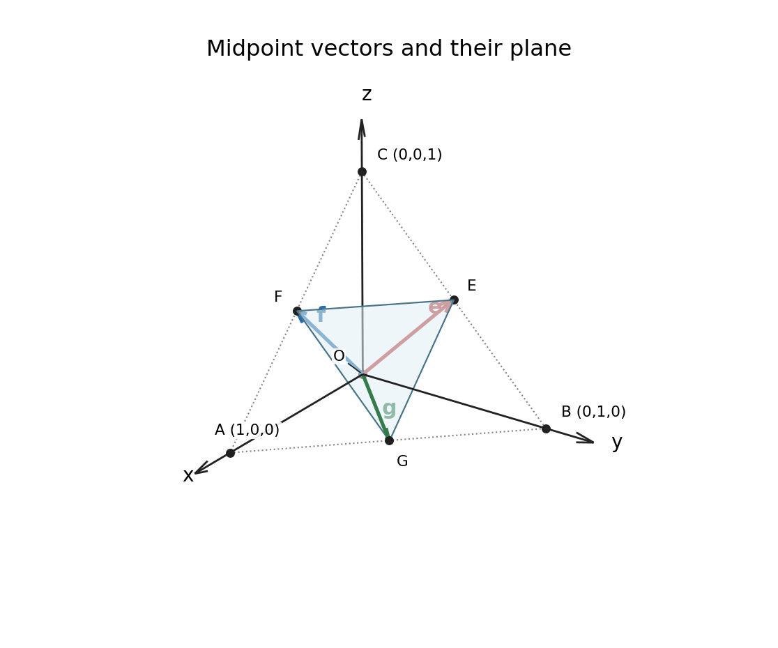
Cartesian axes and three independent midpoint position vectors
. Details. The position vectors end at the midpoints of , and , respectively. The drawing places , and on those edges and shows the arrows from the origin. The volume of their parallelepiped is the absolute scalar triple product:Equivalently, this is the absolute determinant of the matrix whose columns are the three vectors. Since it is nonzero, the vectors are linearly independent. Three linearly independent vectors in the three-dimensional vector space form a basis.
Writing and comparing Cartesian coordinates givesThe unique solution, guaranteed by the basis property, is . Thus
Two directions within the plane areTheir cross product is , so a unit vector normal to the plane isIts negative is equally valid. An equation of a plane through three points in vector form isor, parametrically, . Since the coordinate sum of is one, the Cartesian equation of a plane isThe distance from a point to a plane is the absolute normal displacement, giving
Let . A point on the line has position vector . By bilinearity and antisymmetry of the cross product,For a point with position vector , the area of the parallelogram spanned by and equals base length times perpendicular Euclidean distance. Hence the shortest Euclidean distance to the line isFor , these quantities areThus . The perpendicular meets at , whose displacement from has precisely this length.
The gradient vanishes whenIf , the second equation gives or . If , it gives . These exhaust the possibilities. The stationary points and their values are
The Hessian matrix isAt the origin it is the identity, so the origin is a strict local minimum. At it is , so this point is a saddle point. At either remaining stationary point,which again gives a saddle point. All three saddle points have eigenvalues and ; there are no local maxima.
The most useful guide to the contour plot is the common saddle value. Direct polynomial factorization givesThus the level set is exactly the three complete linesTheir intersections are the three saddle points, and they enclose the origin in an equilateral triangle. Near the local minimum, the level sets are nearly circles because the leading term is . For , a closed contour surrounds the origin, while three separate open branches lie outside the triangular barrier. At the saddle level these components meet at the saddle points; above it the central closed contour has opened into the three outer channels.
The identity in polar coordinatesshows the rotation symmetry through . It identifies the function as the Hénon-Heiles potential and helps organize all three channels in the original sketch below. The dashed straight lines are the saddle level; labels on the other contours give .
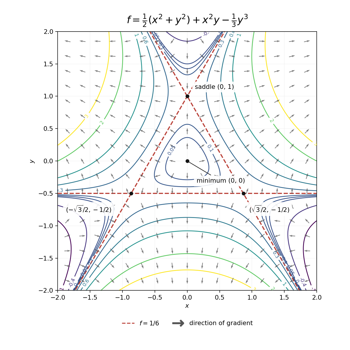
Contours and gradient directions of the Hénon-Heiles potential
. Details. At each regular point, the gradientis normal to the level set and points towards increasing . The arrows in the contour plot above show this direction; their lengths have been normalized to keep the outer arrows legible. Near the origin they point outwards, as expected for a local minimum. Near , write ; the linear approximation is . Thus the arrows point away along the horizontal direction and towards the point along the vertical direction. The other two saddle points have the same behaviour after rotations through . All four stationary points have zero gradient, so no direction arrow is assigned at the points themselves.
A line integral uses , including the tangent vector. With , , the three components sum toConsequently
It is helpful first to separate an exact gradient:The fundamental theorem for line integrals makes the gradient contribution for either path. On the curved path, , , and , so the remaining contribution isThus
A continuously differentiable conservative vector field has zero curl. HereThis vanishes everywhere if and only if . Since the field is smooth on the simply connected domain , zero curl is also sufficient; the explicit scalar potential in the next part confirms it.
With , integrating givesThe other two partial derivatives require . The origin condition fixes the remaining constant to zero. Hence the scalar potential isIts value at gives , so
For a continuous random variable, the probability density integrates to the probability of an interval:Individual endpoints have zero probability, so strict or non-strict inequalities give the same answer.
Subtracting the constant translates the event without changing its probability. ThereforeThis is a translation of the interval in the probability distribution of .
Apply the preceding interval formula on a short interval and use the change of variables :Comparison with the defining integral for a probability density givesAt continuity points, this can also be read as .
The independence of random variables means that fixing leaves the conditional probability density of equal to . Given that value of , is the translate . HenceAt a continuity point of , the expression is . Since , this conditioning uses a conditional probability density, rather than division by the probability of the single event .
Use the law of total probability to average the conditional interval probability over :The integrands are nonnegative, so Tonelli's theorem permits interchanging the integrals. ThusReading off the probability density gives the convolution of probability densities:
A uniform distribution has constant probability density on its interval, and the integral of that density must be one. The interval has length one, soChanging either endpoint value has no effect on the probability distribution.
Insert the two densities into the convolution of probability densities:Using the antiderivative with respect to givesThis is the convolution of a Cauchy distribution and a uniform distribution with half-width .
The probability density is an even function. Its derivative simplifies toIt increases for and decreases for , with maximum height . Thus the most probable value, or mode, is . The original sketch shows the symmetric, slightly flattened peak and long tails.
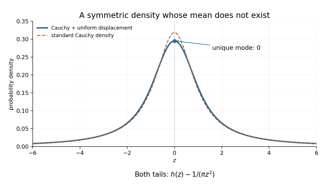


There is a genuine qualification to the request for a mean: the mean does not exist. The integral representation shows that as , soThe two divergent integrals cannot be subtracted to define an expected value. Symmetry does give the Cauchy principal value , but that is not the mean. Equivalently, adding the bounded variable cannot make the first absolute moment of a Cauchy distribution finite.
The characteristic equation of the homogeneous linear differential equation isThe real general solution is . The first boundary value gives . At , and , so . Hence
The characteristic equation has a repeated root , suggesting the substitution . By the product rule,so . The inhomogeneous linear differential equation reduces to . Two integrations giveThereforeThe two arbitrary constants account for the repeated-root homogeneous solution.
The first equation gives . Differentiate it and eliminate using the second equation:Thus the required second-order linear differential equation isConversely, a solution of this equation together with solves both original equations, so the elimination loses no solutions.
The characteristic equation is , with roots . ThereforeIf the second component is also wanted, the relation givesThese are damped oscillations associated with the complex conjugate eigenvalues of the coefficient matrix.
The first initial condition gives . The original first equation gives , whereas the general solution gives . Thus andThe corresponding has , checking the other initial condition.
Articles were limited to the first 100 out of 140 total.
Articles by others on the same topic
There are currently no matching articles.