Past exam of the mathematics course of the year 2 of the natural sciences course of the University of Cambridge / 2007 / Paper 1

Away from the origin, $\hat{\mathbf{r}}=\nabla r$. Hence the curl of a gradient gives $\nabla \times \hat{\mathbf{r}}=0$. Its divergence is the Laplacian of the radial coordinate, which in spherical coordinates isEquivalently, differentiating $x_i/r$ in Cartesian coordinates gives $3/r-r^2/r^3=2/r$.

Use the right-handed orthonormal basis $({\mathbf{e}}_r,{\mathbf{e}}_{\theta },{\mathbf{e}}_{\varphi })$. The cross product with ${\mathbf{e}}_r$ rotates tangential components by a right angle; taking its cross product again in the opposite order projects a gradient onto the tangent plane. The radial curl of angular gradient fields then depends only on the rotated-gradient part. All coordinate calculations are made away from the polar coordinate singularities and extend wherever the original fields are smooth.

Since $\hat{\mathbf{r}}={\mathbf{e}}_r$, the gradient formula givesThe vector triple product identity gives $({\mathbf{e}}_r\times \nabla G)\times {\mathbf{e}}_r=\nabla G-{\mathbf{e}}_r{G}_r=(G_{\theta }/r){\mathbf{e}}_{\theta }+[G_{\varphi }/(r\sin \theta )]{\mathbf{e}}_{\varphi }$. Adding the radial part yields

The radial component of the curl in spherical coordinates isIt contains no $f_r$, so $R$ cannot contribute. Substituting the tangential components givesThe mixed partial derivatives of smooth $G$ agree, so its terms cancel. Multiplication by $r$, to take the dot product with the position vector $\mathbf{r}=r{\mathbf{e}}_r$, does not change this independence from $R,G$.

The remaining terms giveThis is the Laplace-Beltrami operator on the unit sphere. Taking the dot product with the unit radial vector instead would give $r^{-2}{\Delta }_{\theta ,\varphi }F$; the extra factor $r$ here comes from the position vector in the question.

Separation of variables gives $X^{\prime \prime }=-k^{2}X$ and $T^{\prime }=-\kappa k^{2}T$. The periodic matching of both the function and its first derivative selects $k=n\pi /L$, with the constant mode at $n=0$. Thus the periodic diffusion on a circle solution iswhere the Fourier coefficients of the initial function areThe formula for $a_n$ also gives $a_0$ at $n=0$. The constant mode preserves the initial spatial mean; every nonconstant Fourier mode decays. For initial data in L2 space, the series approaches those data in L2 space as $t\downarrow 0$ and is smooth at positive times.

The initial function is odd, so all $a_n$, including $a_0$, vanish. Set $k_n=n\pi /L$. For $k_n\ne 1$, product-to-sum and integration by parts giveConsequently the coefficients of the periodic sine with an endpoint-correcting linear term areInsert them into the sine terms of the preceding solution. If $L=m\pi$ for a positive integer $m$, the original initial profile is simply $\sin x$, with $k_m=1$. The apparent $0/0$ in the displayed coefficient has removable limit $b_m=1$, while $b_n=0$ for $n\ne m$. In that case

Extend $f$ evenly to $F(x)=f(|x|)$ on the whole real line, and use the Fourier transform convention $\hat{F}(k)={\int }_{\mathbb{R}}F(x)e^{-ikx}dx$. Its odd sine contribution vanishes, giving $\hat{F}(k)=2{\int }_0^{\infty }f(x)\cos (kx)dx={\hat{f}}_c(k)$ for $k>0$; the transform is also even. The Fourier inversion theorem therefore gives, for $x>0$,This is the inverse Fourier cosine transform with the factor-of-two forward convention used here.

Take the spatial Fourier transform with the same convention. The partial differential equation becomes $i{\partial }_t\hat{f}-k^2\hat{f}=0$, so $\hat{f}(k,t)=e^{-i{k}^{2}t}{\hat{f}}_0(k)$. Inverting and substituting the transform of the initial function yields the convolutionComplete the square, $iks-it{k}^2=i{s}^2/(4t)-it[k-s/(2t){]}^2$, and put $\ell =\sqrt{t}[k-s/(2t)]$. This givesThe oscillatory Gaussian is a Fresnel integral, understood as the limit with a positive Gaussian damping factor. That prescription also justifies the transform manipulations, first for rapidly decreasing smooth data and then by L2 space extension. The resulting kernel is the free-particle propagator in units $\hslash =1$, $m=1/2$; its phase and normalization agree with the multiplier $e^{-i{k}^{2}t}$.

The matrix trace is $\mathrm{Tr}A={\sum }_i{A}_{ii}$. Expanding the matrix products gives $\mathrm{Tr}(AB)={\sum }_{i,j}{A}_{ij}{B}_{ji}={\sum }_{j,i}{B}_{ji}{A}_{ij}=\mathrm{Tr}(BA)$. Thus the cyclic property of the trace gives zero trace to every commutator. If $AB-BA=I$, taking the trace would give $0=n$, impossible for positive finite $n$ over the real or complex field.

For real $A,B$, let $p(\lambda )=\det (A+\lambda B)$, a real polynomial of degree at most $n$. Since $p(i)=\det C\ne 0$, it is not the zero polynomial. It has at most finitely many real roots of a polynomial, so $A+\lambda B$ is an invertible matrix for some real $\lambda$, in fact for all but finitely many.

Finally write the invertible intertwiner as $R=A+iB$. The relation $PR=RQ$ and the reality of $P,Q$ give $PA=AQ$ and $PB=BQ$. Choose a real $\lambda$ for which $S=A+\lambda B$ is invertible. Then $PS=SQ$, so $P=SQ{S}^{-1}$. This proves that complex similarity of real matrices implies real similarity.

Use the complex inner product $⟨a,b⟩={\sum }_j\overline{a_j}{b}_j=a^{†}b$, conjugate-linear in its first argument. For $a\ne 0$, put $c=⟨a,b⟩/⟨a,a⟩$. Positivity givesHence the Cauchy-Schwarz inequality is $|⟨a,b⟩|\le \Vert a\Vert \Vert b\Vert$. If $a=0$ it is immediate; equality holds precisely when the two vectors are linearly dependent.

For a unitary matrix, $U^{†}U=I$, so $\Vert Ua{\Vert }^2=a^{†}{U}^{†}Ua=\Vert a{\Vert }^2$. If $Uv=\lambda v$ with a nonzero eigenvector, this implies $|\lambda |\Vert v\Vert =\Vert v\Vert$. Thus every eigenvalue satisfiesFor the one-parameter family, expand unitarity to first order: $(I+t{A}^{†}+O(t^2))(I+tA+O(t^2))=I$, so $A^{†}+A=0$. Thus $A$ is a skew-Hermitian matrix, an element of the unitary Lie algebra. If $Av=\mu v$, then $v^{†}Av=\mu \Vert v{\Vert }^2$, whereas complex conjugation gives $(v^{†}Av{)}^{\ast }=v^{†}{A}^{†}v=-v^{†}Av$. Consequently $\overline{\mu }=-\mu$, proving that every eigenvalue of $A$ is purely imaginary, with zero permitted.

Put $s=z-1$ and seek the leading Frobenius series term $y\sim s^{\rho }$. The coefficients of $y^{\prime \prime }$ and $y^{\prime }$ become $-2s(1+s)$ and $2+s$, respectively. The lowest power, $s^{\rho -1}$, therefore has coefficient $-2\rho (\rho -1)+2\rho$. The indicial equation isThe term $-y$ contributes only at the next order and does not enter this equation.

The product rule gives ${\psi }^{\prime }=e^{-x^2/2}(y^{\prime }-xy)$ and ${\psi }^{\prime \prime }=e^{-x^2/2}[y^{\prime \prime }-2x{y}^{\prime }+(x^2-1)y]$. Substituting in the Schrödinger equation cancels the $x^2$ and constant terms, leaving the Hermite differential equationFor $y={\sum }_{n\ge 0}{a}_n{x}^n$, matching coefficients givesThe power series solutions of the Hermite differential equation split into independent even and odd series. With initial data $(y(0),y^{\prime }(0))=(1,0)$ and $(0,1)$, respectively, their first three terms areEach nonterminating parity series has infinite radius of convergence: the ratio of successive terms of that parity has magnitude asymptotic to $2|x{|}^2/n$. Their initial data prove linear independence. If a coefficient shown vanishes at a special parameter, the recurrence supplies the terminating series instead.

A nonzero polynomial solution of degree $N$ requires $\lambda =N$, by its highest-degree term, and the recurrence then terminates the matching parity. Thus all possible values are $\lambda =0,1,2,\dots$. Up to nonzero scalar multiples, the degree-at-most-three solutions are the Hermite polynomials

Multiply the equation for $y_n$ by $y_m$ and the equation for $y_m$ by $y_n$, then subtract. The common $h$ terms cancel, and integration by parts gives the Lagrange identity for a Sturm-Liouville operator:At each endpoint the two pairs $(y_n^{\prime },y_n)$ and $(y_m^{\prime },y_m)$ satisfy the same nontrivial homogeneous linear equation. They therefore lie on the same one-dimensional line, and their determinant vanishes. The boundary expression is zero. Since the eigenvalues are distinct, division gives the required orthogonality of Sturm-Liouville eigenfunctions:For complex-valued eigenfunctions of a real self-adjoint problem one may choose real eigenfunctions, or use the conjugated version as a weighted inner product.

Multiplying by $y$ and integrating with the zero endpoint values first gives $\lambda {\int }_1^b{y}^{2}dx/x={\int }_1^{b}x(y^{\prime }{)}^{2}dx>0$ for a nonzero real eigenfunction; hence $\lambda >0$. Using the printed change of variables $\xi =\lambda \ln x$, write $y(x)=Y(\xi )$. Then $(x{y}^{\prime }{)}^{\prime }={\lambda }^2{Y}_{\xi \xi }/x$, so $Y_{\xi \xi }+Y/\lambda =0$. The first endpoint gives $Y=A\sin (\xi /\sqrt{\lambda })$, and the other gives $\sin (\sqrt{\lambda }\ln b)=0$. ThusThis is the logarithmic change of variable in a Sturm-Liouville problem. The measure $dx/x=d(\ln x)$ gives squared weighted norm $A_n^2\ln b/2$, so an orthonormal choice is $A_n=\sqrt{2/\ln b}$.

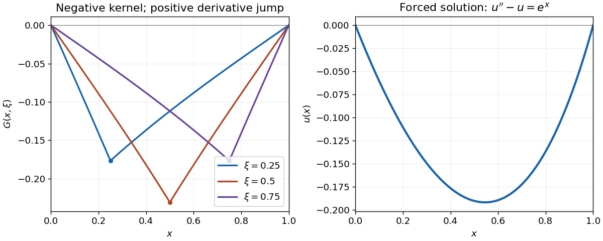
Choose the left homogeneous solution $v(x)=\sinh x$ and the right one $w(x)=\sinh (1-x)$. Their Wronskian is $v{w}^{\prime }-v^{\prime }w=-\sinh 1$. The Dirichlet modified Helmholtz Green function on an interval, with operator sign $D_x^2-1$, is thereforeIt vanishes at both endpoints, is continuous at $x=\xi$, and its first derivative jumps by $+1$, giving $(D_x^2-1)G=\delta (x-\xi )$. The Green-function representation then givesThe two integrals are $(e^{2x}-1)/4-x/2$ and $e(1-x)/2-(e-e^{2x-1})/4$, respectively. Substituting them and simplifying givesDirect differentiation verifies $u^{\prime \prime }-u=e^x$ and both zero boundary values. The negative kernel also explains why the solution is negative inside the interval despite the positive right-hand side.

Take a variation $y_{\epsilon }=y+\epsilon \eta$ with $\eta (a)=\eta (b)=0$. Differentiating the functional at zero and using integration by parts givesThe boundary term vanishes. Since the remaining integral must vanish for every smooth endpoint-zero variation, the fundamental lemma of the calculus of variations gives the Euler-Lagrange equation $d(f_{y^{\prime }})/dx=f_y$.

For the mechanical problem put $A(r)=1-2m/r>0$. The Lagrangian is independent of $\theta$, a cyclic coordinate, so its conjugate momentum $\partial L/\partial \dot{\theta }=2r^2\dot{\theta }=2J$ is conserved. Therefore $J$ is constant, including the factor of two between $J$ and the canonical momentum for this normalization of $L$.

For the radial coordinate, $\partial L/\partial \dot{r}=2\dot{r}/A$ and $\partial L/\partial r=-{\dot{r}}^2{A}^{\prime }/A^2+2r{\dot{\theta }}^2-\mu A^{\prime }/A^2$. Its Euler-Lagrange equation isFor a circular orbit $r=R>2m$, the radial velocity and acceleration vanish. Using $A^{\prime }(R)=2m/R^2$ and $\dot{\theta }=J/R^2$ leaves $2J^2/R^3=2m\mu /[R^{2}A(R{)}^2]$, henceThis is the circular orbit condition for a radial kinetic Lagrangian applied to the coefficients here.

For a nonzero real function, write $\Lambda =F/G$ with $G={\int }_a^{b}w{y}^{2}dx>0$. Multiplying the Sturm-Liouville equation by $y$ and integrating givesThus the stated vanishing boundary product proves $\lambda =\Lambda [y]$.

For the variational statement, the first variation isWith admissible boundary conditions that also make $[p{y}^{\prime }\eta {]}_a^b=0$ for every allowed variation, the fundamental lemma of the calculus of variations identifies stationary functions with the eigenfunctions and stationary values with their eigenvalues. Zero Dirichlet boundary conditions, zero Neumann boundary conditions, and matched periodic data give familiar examples. The single printed condition $[py{y}^{\prime }{]}_a^b=0$ proves the quotient identity but, by itself, does not specify the admissible variations needed for stationarity; the boundary conditions for variational Rayleigh quotients make this distinction explicit.

For the half-line equation, multiplication by $x^{n-1}$ gives $p=w=x^{n-1}$ and $q=x^{n+1}$. Use the regular radial boundary condition at zero and square-integrable decay at infinity, under which the proposed Gaussian is admissible. With $y=e^{a{x}^2}$, $a<0$, $y^{\prime }=2axy$, soThe ratio of the two Gaussian integrals is $n/(-4a)$, from a change of variables and the Gamma function recurrence. Differentiating gives ${\Lambda }^{\prime }(a)=-n[1-1/(4a^2)]$, so the minimum on $a<0$ occurs at $a=-1/2$. The Gaussian variational bound for a radial harmonic oscillator therefore givesHere the trial actually satisfies the differential equation with $\lambda =n$. Moreover, on the same regular decaying domain, integration by parts gives $F[y]-nG[y]={\int }_0^{\infty }{x}^{n-1}(y^{\prime }+xy{)}^{2}dx\ge 0$. Hence the estimate is exact, with $\boxed{{\lambda }_0=n}$. For $n=1$, regular radial data mean the Neumann boundary condition $y^{\prime }(0)=0$; imposing a zero Dirichlet boundary condition there would exclude this trial and give a different problem.