Away from the origin, . Hence the curl of a gradient gives . Its divergence is the Laplacian of the radial coordinate, which in spherical coordinates isEquivalently, differentiating in Cartesian coordinates gives .
Use the right-handed orthonormal basis . The cross product with rotates tangential components by a right angle; taking its cross product again in the opposite order projects a gradient onto the tangent plane. The radial curl of angular gradient fields then depends only on the rotated-gradient part. All coordinate calculations are made away from the polar coordinate singularities and extend wherever the original fields are smooth.
Since , the gradient formula givesThe vector triple product identity gives . Adding the radial part yields
The radial component of the curl in spherical coordinates isIt contains no , so cannot contribute. Substituting the tangential components givesThe mixed partial derivatives of smooth agree, so its terms cancel. Multiplication by , to take the dot product with the position vector , does not change this independence from .
The remaining terms giveThis is the Laplace-Beltrami operator on the unit sphere. Taking the dot product with the unit radial vector instead would give ; the extra factor here comes from the position vector in the question.
Separation of variables gives and . The periodic matching of both the function and its first derivative selects , with the constant mode at . Thus the periodic diffusion on a circle solution iswhere the Fourier coefficients of the initial function areThe formula for also gives at . The constant mode preserves the initial spatial mean; every nonconstant Fourier mode decays. For initial data in L2 space, the series approaches those data in L2 space as and is smooth at positive times.
The initial function is odd, so all , including , vanish. Set . For , product-to-sum and integration by parts giveConsequently the coefficients of the periodic sine with an endpoint-correcting linear term areInsert them into the sine terms of the preceding solution. If for a positive integer , the original initial profile is simply , with . The apparent in the displayed coefficient has removable limit , while for . In that case
Extend evenly to on the whole real line, and use the Fourier transform convention . Its odd sine contribution vanishes, giving for ; the transform is also even. The Fourier inversion theorem therefore gives, for ,This is the inverse Fourier cosine transform with the factor-of-two forward convention used here.
Take the spatial Fourier transform with the same convention. The partial differential equation becomes , so . Inverting and substituting the transform of the initial function yields the convolutionComplete the square, , and put . This givesThe oscillatory Gaussian is a Fresnel integral, understood as the limit with a positive Gaussian damping factor. That prescription also justifies the transform manipulations, first for rapidly decreasing smooth data and then by L2 space extension. The resulting kernel is the free-particle propagator in units , ; its phase and normalization agree with the multiplier .
The matrix trace is . Expanding the matrix products gives . Thus the cyclic property of the trace gives zero trace to every commutator. If , taking the trace would give , impossible for positive finite over the real or complex field.
For real , let , a real polynomial of degree at most . Since , it is not the zero polynomial. It has at most finitely many real roots of a polynomial, so is an invertible matrix for some real , in fact for all but finitely many.
Finally write the invertible intertwiner as . The relation and the reality of give and . Choose a real for which is invertible. Then , so . This proves that complex similarity of real matrices implies real similarity.
Use the complex inner product , conjugate-linear in its first argument. For , put . Positivity givesHence the Cauchy-Schwarz inequality is . If it is immediate; equality holds precisely when the two vectors are linearly dependent.
For a unitary matrix, , so . If with a nonzero eigenvector, this implies . Thus every eigenvalue satisfiesFor the one-parameter family, expand unitarity to first order: , so . Thus is a skew-Hermitian matrix, an element of the unitary Lie algebra. If , then , whereas complex conjugation gives . Consequently , proving that every eigenvalue of is purely imaginary, with zero permitted.
Put and seek the leading Frobenius series term . The coefficients of and become and , respectively. The lowest power, , therefore has coefficient . The indicial equation isThe term contributes only at the next order and does not enter this equation.
The product rule gives and . Substituting in the Schrödinger equation cancels the and constant terms, leaving the Hermite differential equationFor , matching coefficients givesThe power series solutions of the Hermite differential equation split into independent even and odd series. With initial data and , respectively, their first three terms areEach nonterminating parity series has infinite radius of convergence: the ratio of successive terms of that parity has magnitude asymptotic to . Their initial data prove linear independence. If a coefficient shown vanishes at a special parameter, the recurrence supplies the terminating series instead.
A nonzero polynomial solution of degree requires , by its highest-degree term, and the recurrence then terminates the matching parity. Thus all possible values are . Up to nonzero scalar multiples, the degree-at-most-three solutions are the Hermite polynomials
Multiply the equation for by and the equation for by , then subtract. The common terms cancel, and integration by parts gives the Lagrange identity for a Sturm-Liouville operator:At each endpoint the two pairs and satisfy the same nontrivial homogeneous linear equation. They therefore lie on the same one-dimensional line, and their determinant vanishes. The boundary expression is zero. Since the eigenvalues are distinct, division gives the required orthogonality of Sturm-Liouville eigenfunctions:For complex-valued eigenfunctions of a real self-adjoint problem one may choose real eigenfunctions, or use the conjugated version as a weighted inner product.
Multiplying by and integrating with the zero endpoint values first gives for a nonzero real eigenfunction; hence . Using the printed change of variables , write . Then , so . The first endpoint gives , and the other gives . ThusThis is the logarithmic change of variable in a Sturm-Liouville problem. The measure gives squared weighted norm , so an orthonormal choice is .
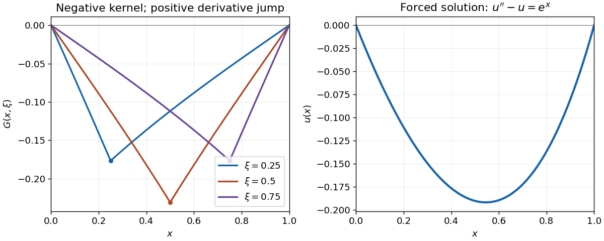
Choose the left homogeneous solution and the right one . Their Wronskian is . The Dirichlet modified Helmholtz Green function on an interval, with operator sign , is thereforeIt vanishes at both endpoints, is continuous at , and its first derivative jumps by , giving . The Green-function representation then givesThe two integrals are and , respectively. Substituting them and simplifying givesDirect differentiation verifies and both zero boundary values. The negative kernel also explains why the solution is negative inside the interval despite the positive right-hand side.

Take a variation with . Differentiating the functional at zero and using integration by parts givesThe boundary term vanishes. Since the remaining integral must vanish for every smooth endpoint-zero variation, the fundamental lemma of the calculus of variations gives the Euler-Lagrange equation .
For the mechanical problem put . The Lagrangian is independent of , a cyclic coordinate, so its conjugate momentum is conserved. Therefore is constant, including the factor of two between and the canonical momentum for this normalization of .
For the radial coordinate, and . Its Euler-Lagrange equation isFor a circular orbit , the radial velocity and acceleration vanish. Using and leaves , henceThis is the circular orbit condition for a radial kinetic Lagrangian applied to the coefficients here.
For a nonzero real function, write with . Multiplying the Sturm-Liouville equation by and integrating givesThus the stated vanishing boundary product proves .
For the variational statement, the first variation isWith admissible boundary conditions that also make for every allowed variation, the fundamental lemma of the calculus of variations identifies stationary functions with the eigenfunctions and stationary values with their eigenvalues. Zero Dirichlet boundary conditions, zero Neumann boundary conditions, and matched periodic data give familiar examples. The single printed condition proves the quotient identity but, by itself, does not specify the admissible variations needed for stationarity; the boundary conditions for variational Rayleigh quotients make this distinction explicit.
For the half-line equation, multiplication by gives and . Use the regular radial boundary condition at zero and square-integrable decay at infinity, under which the proposed Gaussian is admissible. With , , , soThe ratio of the two Gaussian integrals is , from a change of variables and the Gamma function recurrence. Differentiating gives , so the minimum on occurs at . The Gaussian variational bound for a radial harmonic oscillator therefore givesHere the trial actually satisfies the differential equation with . Moreover, on the same regular decaying domain, integration by parts gives . Hence the estimate is exact, with . For , regular radial data mean the Neumann boundary condition ; imposing a zero Dirichlet boundary condition there would exclude this trial and give a different problem.
Put in Laplace's equation, multiply by , and separate the two variables:With , the angular equation becomes . Requiring a smooth axisymmetric harmonic function at both poles selects and the Legendre polynomial , for nonnegative integers . The radial Cauchy-Euler equation has solutions and . Superposition over the angular eigenfunctions therefore givesThis expansion assumes regularity on each whole angular sphere; without it, singular angular solutions would also be possible. The boundary data in the shell involve only the modes. Define the spherical-shell harmonic interpolation weightsEach equals one at the inner boundary and zero at the outer one, and does the reverse. Hence the steady temperature isEach term is a harmonic function, and substitution verifies both prescribed boundary values. Uniqueness follows from the maximum principle for harmonic functions.
For , the radial Laplacian gives . The outward flux of through a small sphere centred at the source is . Applying Green's second identity to a smooth test function outside that small sphere and shrinking its radius therefore gives the distributional identityThe kernel tends to zero at infinity. Thus it is the fundamental solution with the sign convention . The sign will reverse when converting it into the electrostatic potential of a positive point charge through Poisson's equation.
Let be the reflection of the source across the plane. The method of images gives the Dirichlet Green functionThe two source distances agree on , so the boundary value vanishes. The reflected source lies outside the upper half-space, leaving only the required Dirac delta distribution inside. Both terms vanish at infinity.
Put and for . The Dirichlet Green function inside a sphere isOn , the distance identity cancels the two terms. The inverse point lies outside the sphere, so it introduces no interior source. This weighted inversion is the Kelvin transform. For a central source, take the limit to get .
Reflect the source across the equatorial plane and subtract the two ball kernels. This gives the Dirichlet Green function inside a hemisphere . It is zero on the spherical boundary because each ball kernel is zero there, and on the plane because reflection makes their values equal.
For a point charge , Poisson's equation in SI units is , so . Writing for the reflected inverse point givesThe construction uses the real charge, its negative reflected image, a negative inversion image of magnitude , and its positive reflected image. Reflection and inversion commute. All three images lie outside the open upper half-ball, and the prescribed zero boundary values determine the electrostatic potential uniquely.
At a point of complex differentiability, the complex derivative is independent of the direction of approach. Taking increments along the real axis gives ; taking imaginary increments gives . Equality of their real parts and imaginary parts proves the Cauchy-Riemann equations and .
For the specified real part, observe that has exactly that real part. Equivalently, integrating and checking givesThusThe freedom is only a constant imaginary part: the difference of two such holomorphic functions has zero real part, so its Cauchy-Riemann equations make it constant on each connected domain.
The square-root factor gives an algebraic branch point at . The logarithm is locally analytic there but has value an odd multiple of , which is nonzero, so it cannot cancel that branching. The zero and pole of give logarithmic branch points at and , respectively. Thus the finite singularities areInfinity is also a branch point. On the logarithm branch tending to zero there, , so the product behaves as . Other logarithm branches add and retain branching. A chosen branch cut joins or separates these branch points; its ordinary interior points are not additional branch points of the underlying multivalued function.
The denominator factors as . Neither root cancels against the numerator, and both are simple, so the finite singularities areThis is a rational function, so it has no branch points. At infinity, putting gives , analytic at zero; infinity is therefore a removable singularity with value zero.
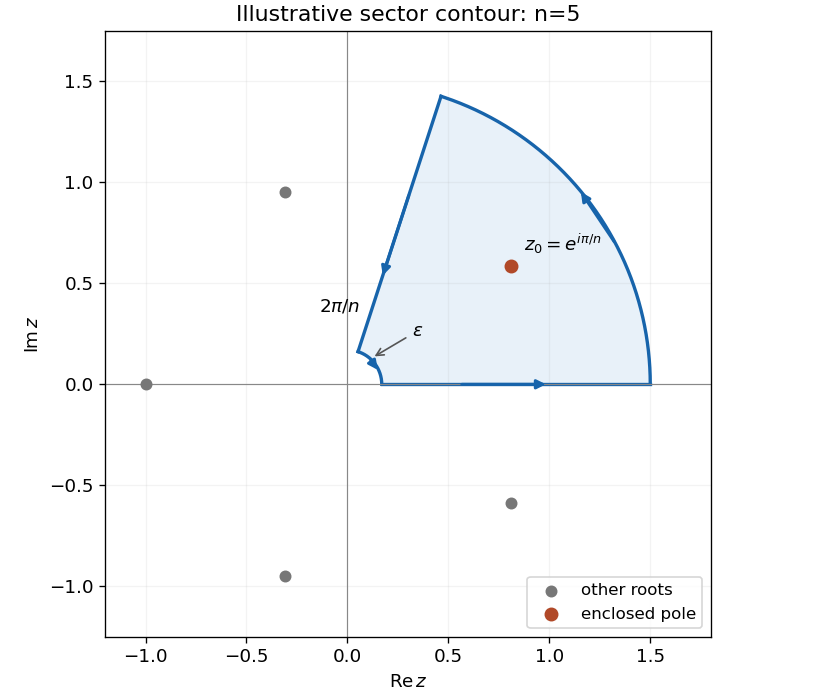
The residue theorem states that the contour integral of a meromorphic function around a positively oriented simple closed contour equals times the sum of its enclosed residues, provided there are no singularities on the contour. The roots of are , . They are simple poles, with residues .
Use the sector contour of angle , running outward along the positive axis and inward along the rotated ray. It encloses only . The large-arc contribution is , hence vanishes. With , the two ray contributions giveSince ,For the second integral, use on a branch continuous across the sector away from zero, with a small inner arc of radius . Its large arc is and its small arc is , both vanishing for . On the rotated ray, changes by , so the two radial contributions add rather than subtract. The enclosed residue is . ConsequentlyBoth answers are instances of the Mellin integral of a reciprocal binomial. The direct contour argument also tracks the branch needed when is odd.

The unilateral Laplace transform is in its region of absolute convergence of a Laplace transform. Under the usual inversion hypotheses, the Bromwich inversion formula isThe vertical Bromwich contour is directed upward, with inside the transform's convergence half-plane and to the right of all its singularities. At discontinuities the standard symmetric inversion gives the mean of the one-sided values.
For a piecewise continuously differentiable with an integrable transformed derivative, integration by parts gives the Laplace transform of a derivative:Here the upper endpoint vanishes by the given decay condition, and right continuity at zero supplies the lower endpoint.
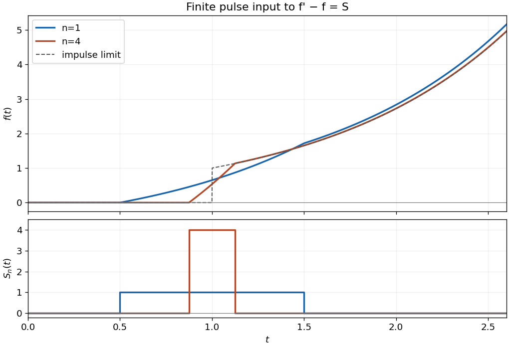
Set , . The finite pulse has Laplace transform . Since , transforming the equation givesThe partial fraction decomposition has inverse . By the Laplace transform time-shift rule,This finite-pulse response of a first-order linear equation gives the requested outer regions:For completeness, while the pulse is active the solution is . It is continuous at both switching times. After the forcing stops it grows as , because the homogeneous equation is . The apparent pole at in the full transform is removable; the Bromwich contour may be taken with .

A two-index Cartesian tensor has components transforming as under an orthogonal change of orthonormal basis. The tensor order here counts indices, rather than the matrix rank. Its scalar, symmetric-traceless and axial tensor decomposition follows by settingThen , with antisymmetric and symmetric and traceless. There are three independent antisymmetric components and five independent symmetric traceless components: three off-diagonal entries and two independent diagonal ones in the latter case.
For the symmetric tensor relative to a nonzero vector , put , , and . The symmetric tensor decomposition relative to an axis givesIn particular . Define the orthogonal projection onto the plane perpendicular to , and setThis tensor is symmetric and kills . Its trace is . To verify the full decomposition, set and split into its longitudinal component , two mixed components, and . The mixed terms are exactly , and gives the longitudinal coefficient. Thus all requested constraints and the reconstruction hold.
For a conservative system near a stable equilibrium, the quadratic Lagrangian has the form , with symmetric mass matrix and stiffness matrix . A normal mode satisfies the generalized eigenvalue problem for small oscillations , so the frequency equation is .
To quadratic order, vertical velocities contribute only fourth-order corrections to the kinetic energy, leaving . A string of length with small horizontal difference shortens its vertical projection by . The upper segment carries all three masses, the middle segment two, and the lower segment one. Hence their increases in gravitational potential energy sum toSubtracting from gives the stated approximate Lagrangian. Here andFor a mode with middle displacement zero, write . The middle row requires , so . A nonzero mode then has , and the outer rows require . Therefore the necessary and sufficient condition isWhen it holds, the mode shape is with . This is the force-cancellation mechanism of the stationary middle mass in a three-mass spring chain, applied to the equivalent quadratic stiffnesses here.
Lagrange's theorem states that the group order of a finite group divides the group order; more precisely .
If every element squares to the identity element, every element is its own inverse element, and . Thus a group of exponent two is abelian. For distinct nonidentity , the four elements are distinct: for example would imply , and would imply . Products remain in this set because commute and square to one. Thus they form a Klein four-group subgroup of order four.
Now let with odd prime number . By Lagrange's theorem, every element order is one of . If an element has order , its square has order . If no element had order , all nonidentity elements would therefore have order two. There are at least two distinct such elements, producing a subgroup of order four. This contradicts . Hence there is an element of order .
A group homomorphism satisfies ; a bijective one is a group isomorphism. Its kernel of a group homomorphism is . It is a subgroup, and for , ,Thus , and applying the same argument to gives equality. Therefore is a normal subgroup.
Write . Direct matrix multiplication gives , and . Consequently these matrices form the integer shear group, a subgroup of . It is an infinite cyclic group, generated by , since and no nonzero integer power is the identity.
The map is a bijective group homomorphism from the additive group of integers, proving the required group isomorphism. There are proper subgroups: for example omits . In fact every subgroup is for an integer , by the classification of subgroups of an infinite cyclic group; gives the trivial subgroup and the whole group.
Substitute and into the quadratic expression. Its coefficients of and are and . The cross term is zero for every matrix in this particular cyclic group, because each has one nonzero entry per row. ThusLet generate the group. For , ; for , . Since , each is its own inverse and . The group law is respected: , and makes it independent of the representative modulo four. This proves that is a group representation.
This quarter-turn action on diagonal quadratic forms hasso it is not faithful. Quadratic forms cannot distinguish a simultaneous sign reversal of both coordinates. The invariant coefficient directions and correspond to the fixed form and the form whose sign changes under a quarter-turn.
Articles by others on the same topic
There are currently no matching articles.