Past exam of the physics B course of the University of Cambridge / 2015 / Paper 1 / Section C

For the attractive inverse-square force, choose zero potential energy at infinity, so $U=-A/r$. At either radial turning point $r_p,r_a$, the kinetic energy is purely tangential, with conserved angular momentum $J$. ThusIts two roots are the periapsis and apoapsis distances. Their sum is $r_p+r_a=-A/E$, whereas the ellipse has $r_p+r_a=2a$. Therefore $a=-A/(2E)$, with $E<0$ for a nondegenerate bound ellipse. The circular case follows by the double-root limit.

For the two-body problem, define $\mathbf{r}={\mathbf{r}}_B-{\mathbf{r}}_A$, total mass $M=m_A+m_B$, reduced mass $\mu =m_A{m}_B/M$, and center of mass $\mathbf{R}$. The relative equation is $\mu \ddot{\mathbf{r}}=\mathbf{F}$, while the isolated center of mass has $\ddot{\mathbf{R}}=0$. Once the relative orbit is known,The relative energy uses $\mu$ in its kinetic energy and $A=G{m}_A{m}_B$ in the gravitational potential energy.

In the equal-mass case the initial relative speed is $u$, $\mu =m/2$, and the center-of-mass velocity is half B's initial velocity. ThusNegative relative energy requires $u^2<4Gm/a_1$. The escape threshold is $u_E=2\sqrt{Gm/a_1}$; equality is marginal parabolic escape, so a strictly bound pair has $u<u_E$.

For $u=u_E/2=\sqrt{Gm/a_1}$, $E_{\mathrm{rel}}=-3G{m}^2/(4a_1)$ and the relative semimajor axis is $a=2a_1/3$. The initial transverse speed is below the relative circular value $\sqrt{2Gm/a_1}$, so the initial turning point is apoapsis. HenceChoose the initial separation along $+x$ from A to B, with B's initial velocity $+u\hat{\mathbf{y}}$. Conservation of angular momentum gives relative periapsis speed $3u$. At the opposite end of the ellipse the direction is $-\hat{\mathbf{y}}$, soThus B has the same speed as initially but the opposite velocity. A has $2u\hat{\mathbf{y}}$ at that instant. A value $3u/2$ for B would be its center-of-mass-frame speed, not the requested initial laboratory frame result.

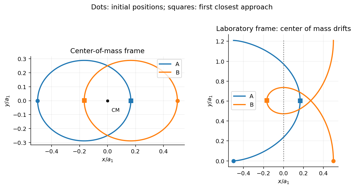
The relative orbital period follows from Kepler's third law with total gravitating mass $2m$:In the center-of-mass frame each star follows an ellipse of semimajor axis $a_1/3$ and eccentricity $1/2$, with the center of mass at a focus; they remain opposite on their simultaneous position vectors. In the laboratory frame add the uniform drift $ut/2$ along $y$. The laboratory paths of an equal-mass binary are therefore not closed ellipses, even though their relative motion repeats.

In Lagrangian mechanics, choose independent generalized coordinates $q_i$ compatible with the mechanical constraints, write $L=T-U$, and apply the Euler-Lagrange equationEquivalently, the physical path makes the action stationary under variations with fixed endpoints. For ideal holonomic constraints, their unknown reaction forces need not appear in the reduced equations. Direct use of Newton's laws of motion instead resolves vector forces and reactions and enforces the constraints separately. Both approaches describe the same mechanics; the scalar Lagrangian is often shorter in curvilinear coordinates. Nonconservative generalized forces must be added separately. Here a drive maintains the prescribed azimuthal angular velocity $\Omega$.

The mass has polar speed $a\dot{\theta }$ and azimuthal speed $a\Omega \sin \theta$, so its kinetic energy is $m{a}^2({\dot{\theta }}^2+{\Omega }^2{\sin }^2\theta )/2$. The elastic potential energy is $\mu {\theta }^2/2$, and the height is $a\cos \theta$, giving gravitational potential energy $mga\cos \theta$. Thereforeand the Euler-Lagrange equation givesFor $\mu =2mga$, define $q={\Omega }^{2}a/g$ and $F(\theta )=q\sin \theta \cos \theta -2\theta +\sin \theta$, so $\ddot{\theta }=(g/a)F(\theta )$. Near zero,When $q<1$ the upright equilibrium is linearly stable and the small oscillations have ${\omega }_1^2=g/a-{\Omega }^2$.

For $q>1$, the graph of $F$ initially rises, whereas $F(\pi /2)=1-\pi <0$. There must therefore be a zero inside the interval. More strongly, for $0<\theta <\pi /2$,is strictly decreasing: $\cos \theta$ decreases and $\theta /\sin \theta$ increases because $\sin \theta -\theta \cos \theta >0$. The ratio goes from $q-1>0$ to $1-\pi <0$, giving exactly one zero ${\theta }_0$ in that interval. At the zero, $F^{\prime }({\theta }_0)<0$, so it is a stable equilibrium. The rotating torsion-stabilized inverted pendulum also has a symmetric stable angle $-{\theta }_0$ if both signs of tilt are permitted.

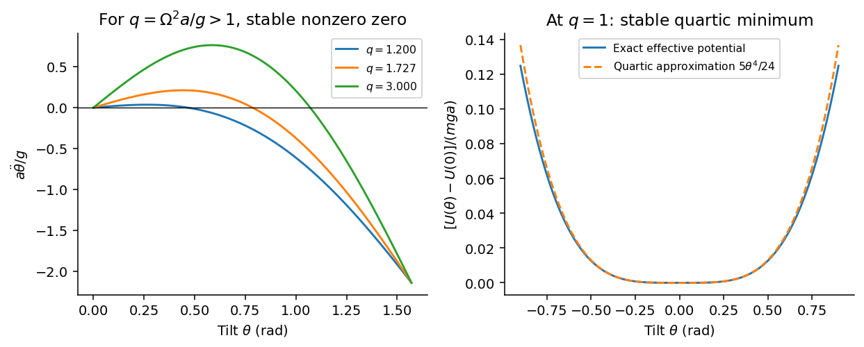
At ${\theta }_0=\pi /4$, setting $F({\theta }_0)=0$ gives $q/2-\pi /2+1/\sqrt{2}=0$, soFor $\theta ={\theta }_0+\xi$, the linearized equation is $\ddot{\xi }=(g/a)F^{\prime }({\theta }_0)\xi$. Since $F^{\prime }=q\cos 2\theta -2+\cos \theta$,At the threshold $q=1$ the linear restoring term vanishes, but the cubic term remains:The upright state remains nonlinearly stable, with no nonzero infinitesimal harmonic frequency. Small finite disturbances produce quartic oscillator motion whose frequency is proportional to its small angular amplitude; its period tends to infinity as that amplitude tends to zero. Zero linear stiffness is not the same as an absent restoring torque.

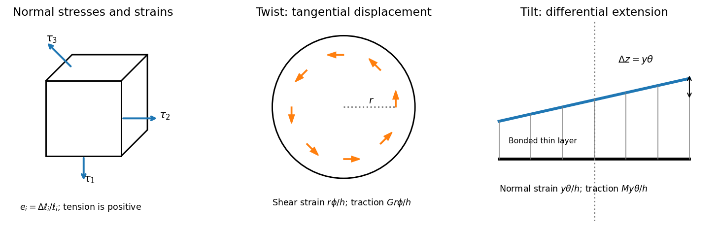
Use positive normal stress for tension. On a small rectangular material element, ${\tau }_i$ is the normal force per unit area on the face perpendicular to axis $i$, and $e_i=\Delta {\ell }_i/{\ell }_i$ is the corresponding normal strain. Young's modulus $E$ is the ratio of axial normal stress to axial strain in uniaxial stress; Poisson's ratio $\sigma$ is minus the transverse-to-axial strain ratio in the same test. Thus isotropic linear elasticity gives $E{e}_1={\tau }_1-\sigma {\tau }_2-\sigma {\tau }_3$ and cyclic permutations. The stress symbols here follow the question; $\sigma$ denotes Poisson's ratio, not a stress component.

For $e_2=e_3=0$, the two transverse compliance equations imply ${\tau }_2={\tau }_3=\sigma {\tau }_1/(1-\sigma )$. Substitution into the first givesThis uniaxial strain modulus is greater than the uniaxial-stress Young's modulus for the positive Poisson's ratio of interest, because the lateral constraints prevent free Poisson contraction.

For a small twist $\varphi$, the bonded faces' relative tangential displacement at radius $r$ is $r\varphi$. The layer's shear strain is $r\varphi /h$, so the shear stress is $Gr\varphi /h$. Integrating the torque givesThe minus sign denotes a restoring torque; the question quotes its magnitude. This uses the disk's polar second moment of area.

For tilt about H, choose $y$ in the plate perpendicular to H. The vertical displacement of the bonded top face is $y\theta$ to first order, giving normal strain $y\theta /h$. The thin layer is constrained laterally by bonding, so its leading normal traction is $My\theta /h$, not $Ey\theta /h$. Integrating its moment about H givessince the diametric second moment of area is $\pi a^4/4$. This is the specified thin-layer approximation to the torsion and tilt stiffness of a bonded elastic disk. Relaxation near the free cylindrical edge is neglected; for a nearly incompressible layer it can limit quantitative accuracy unless the thinness is sufficient.

The thin square plate's moment of inertia about V is $I_V=2m{b}^2/3$. Its two perpendicular in-plane central moments are equal and sum to $I_V$, so the diagonal H has $I_H=m{b}^2/3$. Dividing the two angular stiffnesses by the appropriate moments of inertia givesThe geometry factors cancel in their ratio. Using the supplied relation between shear modulus and Young's modulus,The result lies just below the incompressible isotropic limit $1/2$, as expected for a rubber with a large compression stiffness compared with its shear modulus. It is an inference within the bonded-layer model, rather than an independently measured material constant.

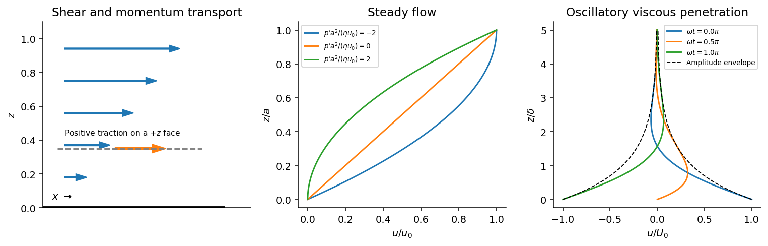
For a Newtonian fluid with velocity $u(z)\hat{\mathbf{x}}$, $\tau =\eta {\partial }_{z}u$ is the $x$ component of traction on a plane whose normal points along $+z$. The opposite face has the opposite traction. The coefficient $\eta$ is dynamic viscosity, with units $\mathrm{Pa}\mathrm{s}$. Faster layers transfer positive $x$ momentum toward slower neighbours; the internal shear stress resists relative sliding.

Take a thin fluid element with horizontal area $A$ and thickness $dz$. The difference between its upper and lower viscous tractions is $A\eta u_{zz}dz$. The pressure gradient supplies $-A{p}_{x}dz$. Incompressibility is satisfied because $u$ has no $x$ dependence, and the convective acceleration vanishes: $(\mathbf{u}\cdot \nabla )\mathbf{u}=u{\partial }_x\mathbf{u}=0$. Equating net force to mass times acceleration therefore gives the relevant component of the Navier-Stokes equation:For steady flow, integrate $\eta u^{\prime \prime }=p^{\prime }$ twice and impose the no-slip boundary condition at each plate, $u(0)=0$ and $u(a)=u_0$. The Couette-Poiseuille flow profile isThe linear term is Couette flow and the parabolic term is plane Poiseuille flow. A negative $p^{\prime }$ drives flow in $+x$. Integrating the profile across the gap gives the volumetric flow per unit width,It has units ${\mathrm{m}}^2{\mathrm{s}}^{-1}$; multiplying by the plate width gives the actual volume per time.

With zero pressure gradient, substituting $u=\mathrm{Re}[A{e}^{i(kz-\omega t)}]$ gives $-i\rho \omega =-\eta k^2$. Select the root that decays into fluid occupying $z>0$:The other sign applies to decay in the opposite half-space. With a real wall velocity amplitude $U_0$, the established periodic solution of Stokes' second problem isThe oscillation's amplitude decays exponentially and its phase lags with distance from the plate. This is diffusion of tangential momentum, not a freely propagating undamped elastic wave. Initial transients must have decayed before this purely periodic expression applies.

The fluid-displacement amplitude and the wall-displacement amplitude have the same ratio as their velocity amplitudes, since both are divided by the common $\omega$. Thus for the specified amplitudes,Using the standard approximate water density $\rho \simeq 10^3\mathrm{kg}{\mathrm{m}}^{-3}$, explicitly an approximation rather than another value printed on the paper, gives $\delta =0.564\mathrm{mm}$ and $z\simeq 2.21\mathrm{mm}$ from either face of a sufficiently large plate. The viscous penetration depth varies as ${\rho }^{-1/2}$ if a more precise water density is used. The ideal parallel-flow solution ignores finite plate edges and tank walls.