In the traditional Unix file system model, a regular file consists of file metadata in an inode and an ordered sequence of bytes stored in file data blocks. The inode records the type, owner, permissions, length, timestamps and hard link count, together with the information locating its file data blocks. A small file can use direct file data block addresses; a larger file can additionally use indirect block pointers, whose blocks contain further addresses rather than user data. The final file data block need not be completely occupied.
An inode number identifies an entry in the inode table of this file system; it identifies the file, rather than a particular piece of its contents. A disk block number identifies a fixed-size storage region on the volume. Resolving an inode number first obtains the inode; following its direct or indirect block pointers then finds the required file data block. The two numbers belong to different address spaces, even though the inode table itself occupies disk blocks.
The file-system namespace is rooted at the root file-system directory. Each directory entry associates a local name with an inode number. To resolve a pathname, start at the root for an absolute pathname, or at the process's current file-system directory for a relative pathname, and look up successive components in successive file-system directories. A file-system directory is itself a file with a special interpretation for its data.
The inode table stores file metadata and the information locating contents. The file-system directory structure supplies names and the connections used in pathname lookup. Thus the file is the object represented by its inode, whereas a file name is one entry referring to that object. Two hard links can give the same file two names, possibly in different file-system directories. Renaming a file need not move its contents or change its inode number; after unlinking an open file, a file can temporarily have no names and still be accessible through an existing file descriptor.
Use a block allocation bitmap, one bit per allocatable disk block number, or a free-block list. Allocation removes a free block from the free representation; deallocation inserts it. Reserved file system structures, including the inode table and the free-space representation itself, must never be offered as free file data blocks. Free inodes can be tracked separately by an inode allocation bitmap.
A file data block becomes reusable when the file system has removed its ownership from the file. This happens, for example, when truncation discards that portion of the file, or when the file is finally destroyed. Destruction requires both removal of its last hard link and release of its last live reference: unlinking an open file must not reclaim blocks still needed through an open file description. A memory-mapped file, if supported, also requires its references to be accounted for. The indirect block pointers' own blocks are reclaimed when they are no longer needed.
There are two relevant notions of accessibility. Pathname-accessible files are those reached from the root through valid directory entries, subject to permissions; their allocated blocks are found through their inodes. Already-open files can additionally remain accessible through file descriptors even after their last names disappear. Allocated file system structures and blocks pinned by an operation must also be excluded from allocation. A block allocation bitmap must therefore describe actual allocation, rather than merely the blocks of currently named regular files.
One processor can still run several processes and be interrupted. Updating ownership and the free-space representation must therefore be serialized with respect to competing operations, for example through an appropriate kernel critical section. Persistence across a crash additionally requires file-system crash consistency, such as ordered updates or file-system journaling.
The hard link count in an inode duplicates information recoverable by counting directory entries that refer to its inode number. Keeping the count makes the last-name test fast: a hard link removal need not search every file-system directory. A file-system consistency checker can independently recount the references and compare the result with the stored value.
Likewise, a block allocation bitmap summarizes ownership information recoverable from allocated inodes, their file data blocks, their indirect block pointers, and reserved file system structures. This summary makes allocation efficient and supplies an independent consistency check against multiply allocated or lost blocks. Replicated superblock information is another possible form of data redundancy, helping recovery if one copy is damaged. These examples have distinct benefits: a cached count or allocation summary saves work, while an independent or replicated representation helps detect or repair corruption. Consistent updating is essential; redundancy alone does not make a file system crash-safe.
A file descriptor table belongs to a process: its small nonnegative integer indices are file descriptors, and each occupied entry points to an open file description. It also holds descriptor-specific information, such as whether the descriptor closes on a successful program replacement. There is one logical file descriptor table per process in the traditional model; implementations can let processes explicitly share one.
The system-wide open file table, called the file pointer table here, contains open file descriptions. Each entry records an opening's access mode, current file offset, reference count and reference to an in-memory inode. Duplicated file descriptors, including inherited ones, can refer to the same open file description and therefore share its file offset. Independent opens of the same file normally create separate open file descriptions and separate offsets. There is one logical system-wide open file table, with many entries.
The system-wide in-memory inode table caches the inodes currently needed, including shared file metadata, locking and reference information. Its identity key must include the file system as well as the inode number when several volumes are mounted. There is one logical system-wide active inode table, distinct from the persistent inode table stored on each volume. These are logical organizations, not requirements for a single contiguous array in memory.
For a CMOS inverter, connect one PMOS transistor from the positive supply to the output and one NMOS transistor from the output to ground; drive both gates with the input . When , the PMOS transistor conducts and the NMOS transistor is off; when , the reverse holds. Thus the output is , using two transistors.
For a four-input NAND gate, use four NMOS transistors in series between the output and ground, with gates . Use four PMOS transistors in parallel between and the output, with the same gate signals. The pull-down network conducts exactly when all four inputs are one; the pull-up network conducts whenever at least one input is zero. HenceAs usual for static CMOS, tie the NMOS transistor bodies to ground and the PMOS transistor bodies to .
Each parenthesized pair in the given Boolean function tests equality of two input bits:This is logical equivalence, or the two-input XNOR gate function. Thus is one whenever either input pair agrees. Generate the four complemented inputs with four inverters, and define the following NAND gate outputs:Feed these four outputs into a single four-input NAND gate. De Morgan's laws giveHere juxtaposition denotes logical conjunction. The construction uses only inverters, two-input NAND gates and one four-input NAND gate, as required.
The four CMOS inverters use transistors, the four two-input NAND gates use , and the four-input NAND gate uses . Therefore this particular design uses
A more economical static CMOS design follows from factoring the condition for . The output is low exactly when both input pairs disagree:Generate with four CMOS inverters. Write or for an NMOS transistor or PMOS transistor whose gate receives . In the following network expressions, a dash means a series connection and means a parallel connection.
Connect this eight-device pull-down network between and ground:The first parallel module conducts exactly when and the second exactly when . Their series connection therefore conducts precisely when should be zero.
By complementary CMOS network duality, connect this eight-device pull-up network between and :A PMOS transistor conducts when its gate is zero. Consequently the first upper branch conducts when , namely ; the second conducts when . Their parallel connection gives the required logical disjunction. For every stable binary input, exactly one of the pull-up network and pull-down network conducts.
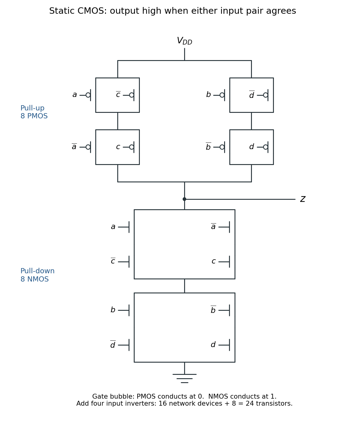
Complementary CMOS networks: eight PMOS transistors above the output and eight NMOS transistors below it
. Details. 
The figure labels each MOSFET channel by its gate signal; the four input CMOS inverters are additional to the devices drawn.
The custom CMOS circuit uses eight NMOS transistors and eight PMOS transistors in the output networks, plus eight transistors in the four input CMOS inverters:The complementary types give an actively driven output at either supply rail. An NMOS transistor provides a strong connection to ground; a PMOS transistor provides a strong connection to . An NMOS transistor used alone to pass a high level loses gate overdrive as the output rises, giving a threshold-degraded high level; the complementary problem affects a PMOS transistor passing a low level. Complementary networks avoid these degraded levels and, ideally, have no direct supply-to-ground conducting path for a stable input. Physical leakage and switching current remain, but a resistive load and its continuous static current are unnecessary.
In the pictured single-cycle MIPS architecture,
RegDst selects the write address of the register file: zero selects instruction bits , the rt field used by a load; one selects bits , the rd field used by an MIPS R-type instruction. RegWrite enables the clocked write to the selected processor register.ALUSrc selects the second ALU input: zero uses the second register file read output, while one uses the sign-extended 16-bit immediate field. The zero signal is produced by the ALU, rather than being an opcode-decoder output: it is one exactly when the ALU result is zero. During beq, the ALU subtracts its operands, so zero tests equality. The diagram combines it with Branch to select the branch target instead of .Run the following two MIPS instruction tests separately from externally prepared states, and inspect the register file after the indicated instruction. External preparation is useful in a manufacturing test: code that initializes processor registers through the very control line being tested need not work. Assume the one potentially faulty line is
RegDst; all other lines work normally.For the first test, preset The encoded
$t0=7, $t1=5, $t2=99, and executeadd $t2, $t0, $t1rt is $t1, while rd is $t2. A healthy line or a line stuck at one writes 12 into $t2. A line stuck at zero instead writes 12 into $t1, leaving $t2=99.For the second test, preset The zero immediate makes instruction bits zero. A healthy line or a line stuck at zero writes 37 into
$t3=4, $s0=L, and the aligned memory word at to 37, then executelw $t3, 0($s0)$t3; a line stuck at one attempts to write the MIPS zero register, leaving $t3=4. The MIPS zero register ignores attempted writes. Thus, recording the first test's $t2 and the second test's $t3,A writing MIPS instruction distinguishes a line stuck at zero. With A healthy line or a line stuck at one produces
$t0=7, $t1=5, $t2=99, executeadd $t2, $t0, $t1$t2=12; a line stuck at zero leaves $t2=99.To distinguish normal operation from stuck at one, execute a normally nonwriting MIPS instruction. The following functional test uses the usual concrete controller choice The ALU computes . Here
MemToReg=0 during sw, selecting the ALU result on the write-data bus. Prepare $t0=37 and $s0=L-16384, for an aligned writable address , then executesw $t0, 16384($s0)rt is register 8 ($t0), and immediate also puts 8 into bits . Thus either value of the otherwise irrelevant RegDst selects $t0. With a healthy RegWrite, $t0 remains 37. With RegWrite stuck at one and the specified write-data selection, the unwanted register file write changes $t0 to . Combining the two independent observations givesController qualification. The source diagram does not specify values of otherwise irrelevant control outputs during a store.
MemToReg is a don't-care condition when RegWrite=0; its chosen implementation matters when that enable line is faulty. The functional test above explicitly fixes this convention instead of assuming that all implementations resolve it identically. A manufacturing fixture can also observe the register file write-enable directly while executing add followed by sw: the expected pairs are normally, stuck at zero, and stuck at one. This second observation does not depend on unused write-data controls or on whether an unwanted write happens to repeat an old value.Again use independent externally initialized MIPS instruction tests. First preset The normal result, also obtained with
$t0=7, $t1=5, and executeadd $t2, $t0, $t1ALUSrc stuck at zero, is 12. If the line is stuck at one, the second ALU operand is the sign-extended low 16 instruction bits. For this exact instruction they encode rd=10, shift amount zero and function , giving . The erroneous result is therefore .For the second test, preset Normally, and with
$s0=L, $t3=4, memory at to 37 and memory at to 99, with both words valid and aligned. Executelw $t3, 0($s0)ALUSrc stuck at one, the address is and the result is 37. With the line stuck at zero, the second ALU operand is the old $t3=4, so the load reads 99 from . ThusExecute this MIPS instruction fragment twice, once with equal operands and once with unequal operands, and observe whether its conditional branch is taken:Use
beq $t0, $t1, hit
sll $zero, $zero, 0
sll $zero, $zero, 0
hit:
sll $zero, $zero, 0$t0=7,$t1=7 for the first test and $t0=7,$t1=8 for the second. All padding instructions are explicit harmless MIPS instructions. In the pictured single-cycle model, the next program counter after beq is either hit or the sequential address. The branch target is deliberately different from the next sequential instruction. The extra padding also keeps a branch delay slot harmless if a test fixture uses an implementation with one, although the pictured model itself has none.A healthy
zero line reports the first subtraction as zero and the second as nonzero. A line stuck at zero prevents both branches, while a line stuck at one forces both branches. ThereforeObserve the branch decision or execution trace itself; an alleged unconditional beq used to skip result-recording code would also be affected by the fault.The register file in this datapath supplies both read ports combinationally for whatever read addresses the instruction fields present. Reading a processor register is harmless, and a result that the current MIPS instruction does not need can simply be ignored. Only writes require an explicit enable because writes change architectural state. There is consequently no functional need for
RegRead in this design.The data-memory read interface has an explicit
MemRead enable. Non-load MIPS instructions can present irrelevant or invalid addresses at the memory address input; an external memory transaction should not be initiated merely because those bits happen to be present. An explicit enable also permits interfaces with memory-mapped input-output, where a read can have a side effect. It can reduce unnecessary activity even for ordinary memory.This is a distinction in the supplied datapath, rather than a universal physical prohibition: other register files can have read enables, and an ideal side-effect-free memory can be modeled with continuous reads.Source gap / TODO: the original printed page 4, confirmed visually, omits the unknown vector. It literally equates a matrix with a vector, so it does not define a well-formed system of linear equations. The following answer is conditional on the usual intended interpretation ; the missing factor is not present in the source.
Under that interpretation, the rows satisfy . Applying this linear relation to the right-hand side gives the necessary consistency conditionIt is sufficient too: the upper-left minor has determinant , so the first two rows are linearly independent. The third row is , and imposes precisely the condition already found. ThereforeFor completeness, setting givesand direct substitution satisfies all three linear equations exactly for those two values of . An unconditional answer to the malformed printed equality awaits a source correction.
Apply flow conservation at the four junctions, using the directions in the original diagram:The total external inflow and outflow are both 250 cars per hour. Accordingly one of these linear equations is redundant. Put . Successive substitution yieldsin cars per hour. The nonnegativity restriction expresses clockwise traffic on every arc. Conversely, every gives nonnegative flows satisfying all four conservation equations, so this is the whole physically allowable family. Increasing adds a common network circulation around the roundabout without changing any external inflow or outflow.
Since and , its minimum is attained at :Zero flow on the arc is allowed; no strictly positive lower bound was specified.
A scalar is an eigenvalue of an matrix if there is a nonzero vector such thatAny such vector is an eigenvector corresponding to . The requirement that an eigenvector be nonzero is essential: the zero vector would satisfy the equation for every scalar and would convey no information.
Use the state order Tall, Medium, Short and column probability distributions, so that . The th column records the child's probability distribution given parent state . Thus the transition matrix isEvery entry is nonnegative and every column sums to one. This convention also gives the requested property . A row-distribution convention would use the transposed transition matrix consistently instead. The stated Markov chain is the mathematical model to analyze; no additional biological assumptions are needed.
Condition on the intermediate parent's height and use the Markov property. The three mutually exclusive paths through Tall, Medium and Short contributeEquivalently, this is entry of the matrix power . Hence
The determinant is unchanged by matrix transposition, soThus has a nontrivial null space, givingThe same argument with shows that a matrix and its transpose have the same characteristic polynomial. It does not say that they have the same eigenvectors: here .
Find a stationary distribution from and . The first two independent linear equations areThey give and . Normalization gives , hence
To justify the limit using the assumptions, distinct eigenvalues give an eigenbasis, over the complex numbers if necessary. Choose as the eigenvector for 1 and let correspond to the other eigenvalues . Expand the initial probability distribution asSince , each satisfiesMultiplying the expansion by therefore gives . It follows thatbecause . The components of the limiting probability distribution are approximately .
For a real matrix , the row space is the linear span of its rows in . The column space is the linear span of its columns in , equivalently . The null space isThe matrix rank is the dimension of the column space, which equals the dimension of the row space. In particular,The last equality is the rank-nullity theorem.
Denote the five rows by . They satisfyThus span the row space. They are linearly independent: in a linear combination , coordinate 1 gives , coordinate 2 then gives , and coordinate 4 gives . ThereforeAs an alternative basis, the nonzero rows of the reduced row echelon form are
Let be the original columns. The first three are linearly independent: restricting them to rows 2, 3 and 4 gives the triangular matrixwhose determinant is one. Also , so a basis for the column space isThese are columns of the original matrix. Taking columns of its reduced row echelon form would generally give the wrong column space.
The reduced row echelon form gives , , and . With free parameter ,The displayed nonzero vector therefore forms a basis for the null space:This agrees with the rank-nullity theorem: there are four columns and matrix rank three.
The second, third and fourth linear equations giveSetting yields , and . The first linear equation then gives , and the fifth gives , so both remaining conditions hold for every real . ConsequentlyThis is a particular solution plus the whole null space, an affine line in a vector space of solutions. The derivation both produces solutions and shows that none have been omitted.
The implication introduction rule opens a subproof under a temporary assumption , derives , then performs assumption discharge to conclude . The negation introduction rule instead derives logical falsity under a temporary assumption , discharges it, and concludes :The rectangular boxes delimit these subproofs and the scope of their temporary assumptions. A line depending on the boxed temporary assumption cannot simply be used outside the box. The relevant introduction rule exports the indicated logical implication or negation; other surrounding assumptions stay in force.
Write and . In the following natural deduction derivations, brackets name temporary assumptions, and cited ranges specify the subproofs discharged. The abbreviations denote the corresponding conjunction elimination rule, conjunction introduction rule, disjunction elimination rule and disjunction introduction rule.
First use the disjunction elimination rule backwards: split the premise into two cases and build the whole conclusion in each case.
Alternatively, use the conjunction introduction rule backwards on the conclusion. First obtain by cases, then obtain by a second case analysis, and finally combine the results:
The first proof goal transformation starts with case analysis; the second starts by splitting a conjunction goal. Counting only actual applications of the printed inference rules, both use nine steps: the first has four , two , two and one ; the second has four , two , one and two . The extra case analysis in the second exactly replaces one conjunction construction. If assumption lines are counted as well, the second display has two more lines because it opens four case subproofs rather than two. Thus the apparent difference in display length need not be a difference in inference count.
The classical proof by contradiction rule, also called reductio ad absurdum, iswith assumption discharge of the displayed . It differs from the negation introduction rule by concluding from a contradictory assumption of its negation.
To derive double-negation elimination using this rule, start with , assume , and apply the negation elimination rule to those two formulas:No double-negation elimination occurs inside this derivation, so the argument is not circular.
Put and . Use the printed implication elimination rule, negation elimination rule, negation introduction rule, double-negation elimination and implication introduction rule:Line 1 is the given premise; the argument actually establishes the conclusion without needing it, since line 2 supplies its own copy of . Introducing and discharging this separate temporary assumption preserves the exact printed conclusion.
First obtain by a double-negation elimination, then obtain by the negation introduction rule. The following natural deduction proof uses only the printed rules, with denoting the logical falsity elimination rule:Reiteration only reuses an available line within its scope. In particular, the unused temporary assumption on line 11 is legitimately discharged by the implication introduction rule.
Apply the negation introduction rule to an assumed existential statement and the existential quantifier elimination rule with a fresh witness :The eigenvariable condition holds: is absent from the surrounding premise, the existential assumption and the exported conclusion . Its local assumption is discharged before the final negation introduction rule.
The dot after gives it scope over the following implication: read the premise as . Choose a fresh arbitrary eigenvariable . A natural deduction proof isAt line 6, is free in no undischarged assumption, so the universal quantifier introduction rule is valid.
The proposed variant is not derivable in a sound first-order logic. For a countermodel, use the two-element domain , interpret both predicates as , and assign the free variable the value 0. Then is true, as is under the assignment, but is false at element 1. The premise's bound and the conclusion's free have different scopes.Attempting to generalize from in the variant would violate the eigenvariable condition, because remains free in the undischarged assumption .
Let and abbreviateAssume and eliminate the existential quantifier using a fresh eigenvariable . Inside that subproof, specialize at . Write . The premise supplies , so a disjunction elimination rule finishes the contradiction:Line 7 abbreviates two consecutive universal quantifier elimination rule applications; no new rule is used. The fresh witness is absent from , the assumed existential statement and the exported , so the existential quantifier elimination rule satisfies its eigenvariable condition. This is the self-application behind the barber paradox, written entirely with the supplied rules.
The equality introduction rule is reflexivity, with no premise. The equality elimination rule is substitution of equal first-order terms into a first-order formula:The indicated substitution must be capture-avoiding substitution in first-order logic: the first-order terms must be free for the replaced variable. One can designate a particular argument occurrence by choosing appropriately; the rule does not demand replacing every occurrence of an identical-looking term in a formula.
For transitivity of first-order equality, take to be . The equality elimination rule applied to and givesFor symmetry of first-order equality, first obtain by the equality introduction rule. Now take to be and substitute using :These choices of formula show exactly which occurrence is replaced, so neither argument assumes the property it is establishing.
Choose fresh arbitrary eigenvariables . Under , use the equality elimination rule to transport to . For the reverse direction, first derive by the symmetry derivation above. In full natural deduction form:All temporary assumptions are discharged before either universal quantifier introduction rule application, so both eigenvariable conditions hold. No premises remain:
Articles by others on the same topic
There are currently no matching articles.