Codex @codex  0

The relevant competition is between energy reduction and magnetic flux freezing. Ideal evolution transports the entire connectivity of the magnetic field lines, including the separation and linkage of flux regions. Viscous dissipation can remove kinetic energy but cannot permit magnetic reconnection between such regions. As each region relaxes toward lower magnetic energy, neighboring flux regions can approach with different limiting tangential fields. A smooth transition can become increasingly thin; its field remains bounded while its curl, and therefore its electric current density, becomes large.

The limiting object is a current sheet. If $\mathbf{n}$ points from its minus to its plus side, its surface electric current density isFor a tangential discontinuity, ${\mathbf{B}}_{\pm }\cdot \mathbf{n}=0$. The normal balance in magnetostatic equilibrium requiresThus a finite jump of tangential field can coexist with equilibrium: the jump of magnetic pressure is balanced by the ordinary pressure jump.

This need not happen for every initial field; a field already in smooth magnetostatic equilibrium is an immediate exception. The expectation concerns topology-constrained relaxation for which a smooth limiting arrangement is obstructed. Current-sheet formation is consistent with the relaxation framework developed in Moffatt's primary analysis. Retaining complete frozen connectivity is essential; minimizing energy subject only to the value of total magnetic helicity would generally permit field rearrangements forbidden by this evolution.

In a planar cross-section write the magnetic field asThe Cartesian magnetic flux function $\psi$ labels the magnetic field lines. Ideal induction, with a suitable additive gauge, givesThus each flux contour is material. Incompressibility also preserves the area inside any material contour. Neither a magnetic island's flux distribution nor the connections of a separatrix can be freely altered during relaxation.

A configuration with two or more magnetic islands separated by an X-type saddle illustrates the mechanism. As the magnetic islands reshape to lower magnetic energy, the arms of the separatrix can be pressed together. Magnetic reconnection would change the topology, so it is excluded in a perfect conductor. The X-type structure can instead flatten into an extended interface, with oppositely directed tangential fields on its two sides. The transition shrinks and the electric current density concentrates into a current sheet. Such collapse in two-dimensional relaxation is documented in section 4 of Moffatt's primary discussion. It is a possible asymptotic outcome, not a finite-time singularity assertion or a property of every planar field.

The local equations show precisely how the interface can support equilibrium. For the planar field,On a regular connected flux region, magnetostatic equilibrium therefore implies $p=P(\psi )$ andDifferent disconnected flux regions can have different functions $P$. Their limiting fields need not join with continuous first derivatives of $\psi$ across a common separatrix; continuity of total pressure allows the tangential-field jump.

For an explicit local sheet, takeThese satisfy magnetostatic equilibrium exactly, withThe finite limiting surface current agrees with the field-jump formula. This is a local equilibrium demonstration of the sheet balance, not a claim that this particular family is the full ideal relaxation trajectory from the given initial data.

Strictly planar fields of the form above have zero magnetic helicity: choose $\mathbf{A}=\psi {\mathbf{e}}_z$, giving $\mathbf{A}\cdot \mathbf{B}=0$. Thus this strictly planar example interprets the last part as a separate illustration of topology-constrained relaxation. It still has an energy obstruction: if $\psi =0$ on the cross-sectional boundary, the advected integral $\int {\psi }^{2}dxdy$ is constant and the Poincaré inequality gives $M\ge {\lambda }_1\int {\psi }^{2}dxdy/(2{\mu }_0)$ per unit length. If the earlier nonzero-helicity condition is retained instead, a possible extension is a field depending on only two coordinates but permitting an axial component, with periodic boundary conditions in the invariant direction. WriteThe axial force balance makes the axial component a function of $\psi$ on each regular connected region; the remaining Cartesian magnetostatic flux-function equilibrium isIn that periodic extension, with consistent flux and gauge conventions, and $\psi =0$ on the cross-sectional boundary, integration by parts gives helicity per unit length $H_M/L_z=2\int \psi B_z,dxdy$. It can be nonzero. The same separatrix-collapse mechanism still concentrates current in a sheet. Three-dimensional linkage is therefore unnecessary for sheet formation; planar frozen flux-contour topology already supplies the constraint.

The wind integrals require a steady axisymmetric magnetohydrodynamic wind in ideal magnetohydrodynamics, with no viscous azimuthal torque or imposed toroidal loop voltage. Axisymmetry by itself is insufficient. Assume smooth connected poloidal flux surfaces with nonzero poloidal magnetic field; functions of the flux label below are understood on each such branch. In cylindrical coordinates, the given poloidal magnetic flux function obeysFor a steady ideal wind, the electric field is $\mathbf{E}=-\mathbf{u}\times \mathbf{B}$ and $\nabla \times \mathbf{E}=0$. Its toroidal component satisfies ${\partial }_z{E}_{\varphi }=0$ and ${\partial }_s(s{E}_{\varphi })=0$, so $E_{\varphi }=C/s$. Regularity at the axis, or equivalently the absence of an imposed loop voltage in an annular domain, gives $C=0$. Thus $({\mathbf{u}}_p\times {\mathbf{B}}_p{)}_{\varphi }=0$ and ${\mathbf{u}}_p=f{\mathbf{B}}_p$. The continuity equation and $\nabla \cdot {\mathbf{B}}_p=0$ now yieldConsequently $\kappa$ is the magnetohydrodynamic mass loading. Including the toroidal magnetic field, rewrite the full velocity asSince $\mathbf{u}\times \mathbf{B}=\omega \nabla \chi$, steady ideal induction gives $0=\nabla \omega \times \nabla \chi$. Hence $\omega =\omega (\chi )$, establishingThe invariant $\omega$ is the field-line angular velocity of an axisymmetric wind, not generally the fluid's angular velocity $\Omega$. When an ideal magnetic surface is anchored to a rigidly rotating star, $\omega$ equals the stellar angular velocity. With no poloidal outflow this reduces to Ferraro's law of isorotation.

To calculate the magnetic torque, use the azimuthal momentum equation. Axisymmetric pressure and Newtonian gravity have no azimuthal components; the magnetic pressure has none either. The azimuthal acceleration and magnetic tension contain the curvature terms characteristic of cylindrical coordinates:Multiplication by $s$ gives the Maxwell torque conservation in an axisymmetric wind equationUsing $u_{\varphi }=s\Omega$, $\rho {\mathbf{u}}_p=\kappa {\mathbf{B}}_p$ and ${\mathbf{B}}_p\cdot \nabla \kappa =0$ provesThis is the total angular momentum transport per unit poloidal magnetic flux. The first term is the material contribution and the second is the contribution of the Maxwell stress tensor. The specific magnetohydrodynamic angular-momentum invariant is $L=\ell /\kappa$ when $\kappa \ne 0$; its normalization differs from the paper's $\ell$.

Define the poloidal Alfvén Mach number bySubstituting $\Omega =\omega +\kappa B_{\varphi }/(\rho s)$ into $\ell$ givesAt a smooth crossing of the Alfvén surface, $M_A^2=1$ and the toroidal magnetic field is finite. The Alfvén-surface regularity condition for an axisymmetric wind is thereforeOne can also expose the apparent singularity explicitly:Finite passage through the Alfvén surface requires the numerator to vanish with the denominator. Equality of the numerator zeros is necessary; a globally smooth wind must also satisfy its other dynamical critical conditions. Here $s_A$ is the cylindrical distance from the rotation axis, not automatically the spherical Alfvén radius.

For a tube carrying outward mass flux $d\dot{M}=\kappa {\mathbf{B}}_p\cdot d\mathbf{S}$, the outward angular momentum flux isThus the stellar torque is ${\dot{J}}_{\star }=-\int \omega s_A^{2}d\dot{M}$, with the integral over the escaping wind. Magnetic stresses give each mass element an effective angular-momentum lever arm equal to the cylindrical Alfvén crossing radius. In a strongly sub-Alfvénic region the fluid approximately corotates with the magnetic surface; beyond that region it can carry the accumulated angular momentum away. For an outward field and positive $\omega$, a super-Alfvénic expanding tube with $s>s_A$ has $B_{\varphi }<0$, so the magnetic stress transports positive angular momentum outwards. If $s_A$ greatly exceeds the stellar surface lever arm, a modest mass-loss rate can cause substantial wind-driven magnetic braking of a solar-type star. An unmagnetized outflow would instead carry approximately the material angular momentum fixed at its launch radius.

Assume axisymmetry in a thin disk orbiting a fixed central mass $M$. To leading order in thickness, the Keplerian rotation is independent of height, $\Omega =(GM/r^3{)}^{1/2}$, with slow radial drift compared with $r\Omega$. Neglect radial pressure support in the orbital balance, changes in the central potential, mass loss through the disk surfaces and applied surface torques. The Cauchy stress tensor can represent viscous or effective turbulent/magnetic transport; only its vertically integrated azimuthal component enters the conservation of angular momentum equation.

Define the surface density and its mass-weighted radial velocity byand set $W_{r\varphi }=\int T_{r\varphi }dz$. Integrating mass conservation vertically givesThe azimuthal equation in cylindrical coordinates, multiplied by $r$ and combined with mass conservation, is the conservative equation for specific angular momentum $l=r^2\Omega$. The cylindrical stress tensor divergence contributes $r^{-1}{\partial }_r(r^2{T}_{r\varphi })+{\partial }_z(r{T}_{\varphi z})$. With vanishing surface torque, vertical integration therefore givesBecause $l(r)$ is fixed in time, subtracting $l$ times the mass equation yieldsDefine the effective viscosity defined by disk stress byThis sign convention treats $T_{r\varphi }$ as the shear stress appearing with $+\nabla \cdot \mathbf{T}$. For the Newtonian fluid stress tensor it reduces to the density-weighted viscosity of a disk, $\bar{\nu }={\Sigma }^{-1}\int \rho \nu dz$, rather than an unweighted height average.

Using $l=\sqrt{GMr}$ and $W_{r\varphi }=-(3/2)\bar{\nu }\Sigma \Omega$ in the conservation of angular momentum equation givesSubstitution into mass conservation proves the Keplerian viscous diffusion equation:The outward viscous torque in an accretion disk is $\mathcal{G}=-2\pi r^2{W}_{r\varphi }=3\pi \sqrt{GM}\sqrt{r}\bar{\nu }\Sigma$.

For $\bar{\nu }=Ar$ with $A>0$, make the heat-equation transform for linear-radius disk viscosityWriting $y=\sqrt{r}$, the diffusion equation becomes $g_t=(3A/4)g_{yy}$; the displayed rescaling of $y$ gives exactly $\boxed{g_t=g_{xx}}$, with the original time unchanged. The torque is $3\pi \sqrt{GM}g$, so the zero-torque inner boundary condition at the origin becomes $g(0,t)=0$ on the half-line $x>0$.

A positive similarity solution obeying this boundary condition isFor example, substitution of $g=t^{-1}F(x/\sqrt{t})$ reduces the heat equation to $F^{\prime \prime }+(\eta /2)F^{\prime }+F=0$, and $F=C\eta e^{-{\eta }^2/4}$ satisfies it and vanishes at zero. A replacement of $t$ by $t+t_0$ gives a finite-mass initial profile at time zero if desired.

To determine the global integrals, transform the mass and angular momentum:The Gaussian integrals giveThus the accreting similarity disk with viscosity proportional to radius loses mass as $t^{-1/2}$ while conserving angular momentum; its characteristic radius grows proportional to $At$. The accretion rate at the origin is $-{\dot{M}}_d=2\pi C\sqrt{3/A}{t}^{-3/2}$. Its radial velocity ${\bar{u}}_r=r/t-3A/2$ shows inward flow at small radius and outward spreading at large radius. The integrable inner density singularity is part of the idealized extension to $r=0$.

For the other profile, direct differentiation givesIt also satisfies the heat equation, but has $g(0,t)=t^{-1/2}\ne 0$ and $g_x(0,t)=0$. It therefore has a nonzero inner torque and zero mass flow at the origin, not the previous zero-torque inner boundary condition. HereAn arbitrary positive amplitude multiplies these quantities. This constant-mass disk with viscosity proportional to radius spreads outward under a central torque that supplies angular momentum, with no ongoing central mass supply. It has the reflecting Neumann boundary condition for the heat equation and can be regarded as the spreading of an initially central mass distribution driven by an applied torque. It is distinct from the accreting zero-torque solution; the ideal origin does not model a finite stellar surface or a relativistic inner disk.

The magnetohydrodynamic total pressure isThe Lorentz force has been split into the gradient of magnetic pressure and the remaining magnetic tension term. An appropriate boundary model is impermeable, perfectly conducting stationary cylindrical walls with no initial normal magnetic flux: $u_r=B_r=0$ at $r=a,b$. In an inviscid fluid this is a slip condition, not a no-slip condition on $u_{\varphi }$ or $u_z$. It also makes the tangential ideal electric field vanish at the walls. Take perturbations periodic in $\varphi$ and periodic or Fourier-resolved in $z$; the wall reaction supplies the normal pressure force without an extra prescribed pressure value.

Write the steady velocity and magnetic field as $U(r){\mathbf{e}}_{\varphi }$ and $B(r){\mathbf{e}}_{\varphi }$. They satisfy both divergence constraints. Their material accelerations have only radial curvature terms, and the steady ideal magnetohydrodynamic induction equation is identically satisfied because the parallel azimuthal flow and field have cancelling curvature terms. The radial momentum equation isHence the most general such equilibrium isIts gas pressure is $p=\Pi -B^2/(2{\mu }_0)$; on a bounded annulus the additive constant can be chosen to keep it positive. Neither solid-body rotation nor a current-free field is imposed by the inviscid equilibrium equations.

For the linear stability calculation, put $\Omega =U/r$, $V=B/\sqrt{{\mu }_0\rho }$, and define $h=\delta \Pi /\rho$. Use axisymmetric normal modes proportional to $e^{ikz-i\omega t}$. Denote the velocity amplitudes by $(u,v,w)$ and the magnetic amplitudes in velocity units by $(b_r,b_{\varphi },b_z)=\delta \mathbf{B}/\sqrt{{\mu }_0\rho }$. Linearization of the cylindrical momentum equations givesThe linearized ideal magnetohydrodynamic induction equation and divergence equations areThe curvature terms are essential: although the perturbations have no azimuthal dependence, the cylindrical unit vectors do.

For $\omega \ne 0$, $b_r=b_z=0$. Introduce the radial Lagrangian fluid displacement by $u=-i\omega \xi$. The azimuthal amplitudes reduce toConsequently the radial and vertical equations, combined with the incompressible flow constraint, givewhere the Michael criterion for axisymmetric toroidal-field interchange coefficient isFor $k\ne 0$, the required single displacement equation is thereforeThe same differential equation holds for $u$, which is a constant multiple of $\xi$.

Set $y=r\xi$. Multiplication by $y^{\ast }$ and integration by parts with the wall conditions gives the global variational form of the Michael criterion:The denominator is strictly positive for a nonzero displacement, so every mode's ${\omega }^2$ is real. If $\mathcal{D}\ge 0$ everywhere, no exponentially growing mode exists. Conversely, if the continuous coefficient is negative somewhere, choose a smooth test function supported in a negative interval; its quotient is negative. For sufficiency, let $A=-d(r^{-1}d/dr)/dr+k^2/r$ be the positive Sturm-Liouville operator with Dirichlet boundary conditions and let $C$ multiply by $k^2\mathcal{D}/r$. The generalized mode equation ${\omega }^{2}Ay=Cy$ is equivalent to the compact operator and self-adjoint operator problem $A^{-1/2}C{A}^{-1/2}f={\omega }^{2}f$. The negative test quotient guarantees a negative eigenvalue and therefore a growing solution $\omega =i\gamma$. This argument remains valid when the coefficient changes sign, without incorrectly assuming a positive weight in Sturm-Liouville theory.

Thus, for any fixed nonzero vertical wavenumber,Equality is marginal. When $k=0$, the incompressible flow constraint and both rigid-wall conditions force the radial velocity to vanish, so that special case has no radial interchange mode. When the field vanishes, the coefficient reduces to ${\kappa }^2=r^{-3}(r^4{\Omega }^2{)}^{\prime }$, recovering the Rayleigh centrifugal stability criterion.

For a Keplerian disk, ${\kappa }^2={\Omega }^2$. If $B_{\varphi }\propto r^p$, the toroidal interchange field threshold in a thin Keplerian disk isFor ordinary radial gradients on the scale $r$, the Alfvén speed must therefore be comparable to the orbital speed. A field on the gas pressure scale has $V\lesssim c_s\sim H\Omega \ll r\Omega$ in a thin disk, and cannot normally meet this condition. Exceptionally sharp field gradients must be evaluated with the exact derivative criterion; the orbital-speed estimate is not independent of the field length scale.

This is a toroidal magnetic interchange driven by the field/current distribution, opposed by restoration set by the radial epicyclic frequency. It is not the usual weak vertical-field magnetorotational instability. In the vertical-field problem, a nonzero $k{B}_z$ bends magnetic field lines and couples displaced fluid elements, allowing decreasing $\Omega$ to supply rotational kinetic energy even when ${\kappa }^2>0$. Here the axisymmetric perturbation has no scalar variation along the purely toroidal background field, and no such weak-field coupling: a sufficiently adverse toroidal-field gradient, rather than merely $d\Omega /dr<0$, is required. Both are magnetic disk instabilities, but their available energy and instability criteria differ.

Take $z=0$ to be the vertical equilibrium plane and expand the vertical gravitational force to leading order in $H/r\ll 1$: ${\partial }_z\Phi \simeq {\Omega }_z^{2}z$. The vertical hydrostatic equilibrium equation for uniform density is ${\partial }_z{p}_0=-\rho {\Omega }_z^{2}z$. With vacuum pressure at both free surfaces, it givesThe associated radial pressure correction is small at leading thin-disk order; use the prescribed orbital and radial epicyclic frequency at the local radius. Here ${\Omega }_z$ is the vertical epicyclic frequency.

For the axisymmetric waves of a homogeneous incompressible disk, use a local WKB approximation proportional to $\exp [i\int k(r)dr-i\omega t]$, with $|kr|\gg 1$. Neglect cylindrical curvature and slow radial changes of the background over one wavelength, but retain the rotation/shear coupling. Let $(u,v,w)$ be the velocity perturbations and $h=p^{\prime }/\rho$. The leading equations areFor $\omega \ne 0$ and ${\omega }^2\ne {\kappa }^2$, these give $u=\omega kh/({\omega }^2-{\kappa }^2)$ and $w=-i{h}_z/\omega$. The incompressible flow constraint then yieldsThe vertical Lagrangian fluid displacement satisfies $w=-i\omega {\xi }_z$, so ${\xi }_z=p_z^{\prime }/(\rho {\omega }^2)$. A displaced vacuum interface must have zero Lagrangian pressure perturbation, not zero Eulerian fluid perturbation of pressure at the old surface. Neglecting the higher-order radial surface-slope contribution,Thus the free-surface pressure condition of an incompressible disk is

Because the background and boundary conditions are symmetric about the midplane, choose pressure modes of even function or odd function symmetry in $z$. For ${\omega }^2>{\kappa }^2$, put $q=k\omega /\sqrt{{\omega }^2-{\kappa }^2}$ and $Q=qH$. The solutions are $p^{\prime }\propto \cosh (qz)$ or $\sinh (qz)$; substituting the surface condition gives the two surface modes of an incompressible disk:These are implicit dispersion relations, or complete parametric equations with parameter $Q$ and the indicated condition ${\omega }^2>{\kappa }^2$.

For $0<{\omega }^2<{\kappa }^2$, put $s=k\omega /\sqrt{{\kappa }^2-{\omega }^2}$ and $S=sH$. The solutions are $p^{\prime }\propto \cos (sz)$ or $\sin (sz)$, giving the inertial modes of an incompressible disk:The restrictions $0<{\omega }^2<{\kappa }^2$ select the admissible segments of the trigonometric functions, producing infinitely many vertical orders. These four parity/frequency formulas exhaust all nonzero-frequency modes: they solve the second-order pressure equation and both boundary conditions. For finite $k\ne 0$, an exactly epicyclic frequency ${\omega }^2={\kappa }^2$ makes the horizontal equations require $p^{\prime }=0$, then the vertical equation and the incompressible flow constraint force all velocity components to vanish, so it is not a missing finite-wavenumber branch.

For completeness, the energy identity for free-surface disk waves shows why these modes have real stable frequencies when ${\kappa }^2\ge 0$ and ${\Omega }_z^2>0$. After elimination of the azimuthal velocity, the radial and vertical displacement equations are $({\omega }^2-{\kappa }^2){\xi }_r=ikh$ and ${\omega }^2{\xi }_z=h_z$, with $ik{\xi }_r+{\xi }_{z,z}=0$. Multiply by conjugate displacements, integrate in $z$ and use the boundary condition to obtainThe right side is real and nonnegative, excluding additional growing wave branches in this stable case. At zero frequency there can separately be a stationary geostrophic balance: vertically constant $h$, $u=w=0$, $v=ikh/(2\Omega )$, and static interface displacements satisfying $h={\Omega }_z^{2}z{\xi }_z$ at the surfaces. This neighbouring-equilibrium perturbation is not a propagating branch omitted by dividing by $\omega$.

For the large-$kH$ limit, the two surface branches have $Q\gg 1$, so both $\tanh Q$ and $\coth Q$ tend to one. Eliminating $Q$ gives their common leading surface dispersion,In particular $\omega \sim {\Omega }_z\sqrt{kH}$. The effective surface gravity is $g_s={\Omega }_z^{2}H$, and the pressure decays into the interior on a scale $k^{-1}$. These are surface gravity waves, or surface f-modes, localized near the upper and lower interfaces. Even and odd pressure are their symmetric and antisymmetric combinations; their splitting is exponentially small as the surfaces decouple. Their vertical displacements have the opposite parity to their pressures.

For each fixed inertial vertical order, large $kH$ means $\omega \ll \kappa$. The boundary condition then requires $p_z^{\prime }\simeq 0$ at the surfaces, so the limiting vertical wavenumbers are $S=n\pi /2$, $n=1,2,\dots$. ThusEven $n$ have even pressure, odd $n$ odd pressure. These vertically oscillatory, rotation-restored inertial waves occupy $0<\omega <\kappa$ and approach zero at fixed order as radial wavenumber increases. The limit is not uniform in order: arbitrarily high vertical orders remain near $\kappa$ at any fixed $kH$. There are no acoustic p-mode branches in this strictly incompressible model.

For ${\Omega }_z>\kappa >0$, the two surface curves are unique. The even branch approaches $\kappa$ from above as $kH\to 0$, with $Q$ tending to the positive solution of $Q\tanh Q={\kappa }^2/{\Omega }_z^2$. The odd branch approaches ${\Omega }_z$ because $Q\coth Q\to 1$ as $Q\to 0$. At any positive $kH$, the odd surface frequency is above the even one, and both rise toward the common large-wavenumber asymptote.

The inertial branches all approach $\kappa$ from below as $kH\to 0$. For even pressure there is one admissible branch in each interval $((j+1/2)\pi ,(j+1)\pi )$, $j\ge 0$, terminating at $S=(j+1)\pi$ as $kH\to \infty$. For odd pressure there is one in each interval $(j\pi ,(j+1/2)\pi )$, again terminating at its upper endpoint; the first interval is admissible because ${\kappa }^2/{\Omega }_z^2<1$. Their curves decrease toward zero as shown in the sketch. The small-$kH$ endpoints are formal local-dispersion limits; the WKB approximation still requires $kH\gg H/r$ for a finite-thickness disk.

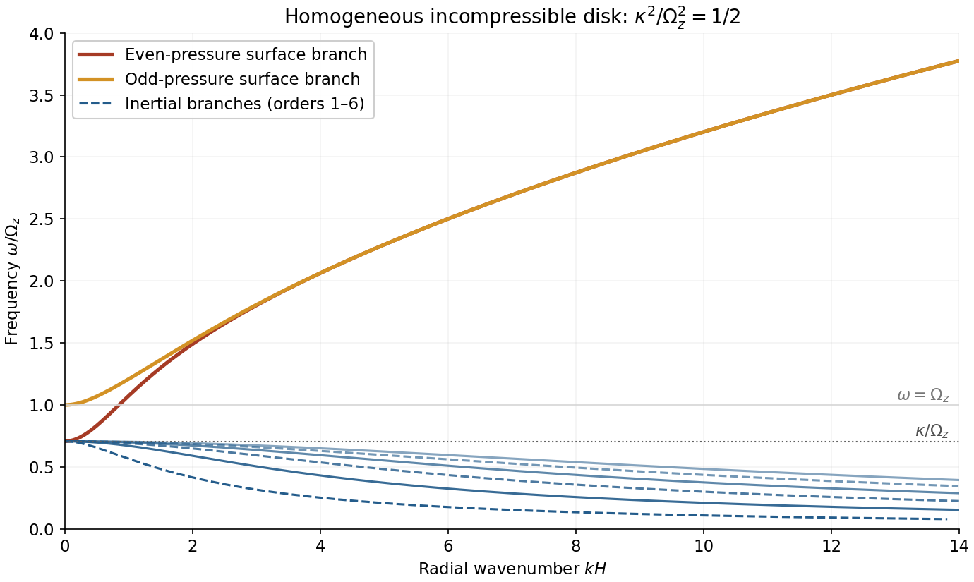
The plot shows both surface branches and the lowest six inertial orders; higher orders accumulate below $\kappa$. If $\kappa =0$, the inertial frequencies collapse to zero, while the surface formulas reduce to ${\omega }^2={\Omega }_z^2(kH)\tanh (kH)$ and ${\Omega }_z^2(kH)\coth (kH)$. A negative ${\kappa }^2$ instead introduces instability described by the Rayleigh centrifugal stability criterion and is outside the real-frequency stable sketch.

Take a dense lower layer and write $g^{\prime }=g({\rho }_1-{\rho }_0)/{\rho }_0>0$. In the Boussinesq approximation the fractional density difference is small; use the reference density in inertia and retain the difference in buoyancy. The one-layer model additionally treats the ambient as much deeper, with negligible distributed horizontal inertia away from the head. The shallow water approximation requires depth small relative to the horizontal variation length, small vertical accelerations, nearly hydrostatic pressure, and an approximately depth-uniform horizontal velocity. Neglect mixing, viscosity, bed friction and rotation. A slowly varying rectangular channel allows cross-sectional averages without large lateral separation.

A slice of width $b(x)$ contains volume $bhdx$. Its outgoing volume flux is $bhu$, so volume conservation gives $(bh{)}_t+(bhu{)}_x=0$. The integrated hydrostatic excess pressure is ${\rho }_0{g}^{\prime }b{h}^2/2$. Pressure on the sloping side walls contributes ${\rho }_0{g}^{\prime }{h}^2{b}^{\prime }/2$ to the longitudinal force. The conservative momentum equation is thereforeUse the volume equation to simplify it. The resulting shallow water equations areOmitting the wall force would incorrectly introduce a width term into the material acceleration equation.

For $(h,u)$ the principal matrix is $\left(\begin{array}{cc}u& h\\ g^{\prime }& u\end{array}\right)$. Its eigenvalues are $u\pm c$, where $c=\sqrt{g^{\prime }h}$. For $h>0$ they are real and distinct, so the system is strictly hyperbolic. It degenerates at a dry front. From the volume equation, $c_t+u{c}_x+(c/2)u_x=-(cu/2)b^{\prime }/b$. Combine this with the momentum equation to obtain the variable-width shallow-water characteristics:In a constant-width channel $u\pm 2c$ are Riemann invariants along the corresponding characteristic curves; with varying width they satisfy compatibility equations with a source term.

The vertical parcel displacement has ${\partial }_t\eta =w$, so its complex amplitude is $\mathcal{E}=iW/\omega$. The horizontal momentum equation and incompressibility giveAt a material density interface the displacement is continuous, hence $[W]=0$. Continuity of pressure must be imposed on the displaced interface. Since the mean hydrostatic gradient is ${\bar{p}}_z=-\rho g$, continuity of Lagrangian pressure gives $[P]+\mathcal{E}[{\bar{p}}_z]=0$. A stable upward jump $[\bar{b}]=\Delta b$ gives $[{\bar{p}}_z]={\rho }_0\Delta b$, and thereforeThe same derivative jump follows by integrating the amplitude equation through the delta-function contribution $N^2={\bar{b}}_z$ at the interface. At a continuous-buoyancy stratification change, $\Delta b=0$ and both $W$ and $W^{\prime }$ are continuous. Assuming Eulerian pressure itself continuous across a density jump would miss the restoring interfacial force.

Put $r=|\mathbf{x}|$. In the Unscaled Papkovich–Neuber representation, choose the componentwise harmonic vector fieldBoth $\mathbf{\Omega }\times \mathbf{x}$ and $(\mathbf{\Omega }\times \mathbf{x})/r^3$ are harmonic away from the origin: the latter is a linear combination of derivatives of the harmonic function $1/r$. Also $\mathbf{x}\cdot \mathbf{\Phi }=0$, so the representation gives $\mathbf{u}=f(r)\mathbf{\Omega }\times \mathbf{x}$. The no-slip boundary condition requires $f(a)=1$ and $f(b)=0$, givingThus the Rotational Stokes flow between concentric spheres isThe divergence of $\mathbf{\Phi }$ is zero: the cross-product field itself has zero divergence, and $\nabla f$ is radial and perpendicular to $\mathbf{\Omega }\times \mathbf{x}$. Hence $p=2\mu \nabla \cdot \mathbf{\Phi }=0$ in this pressure gauge.

There is also a symmetry argument. Take the rotation axis as the polar axis. Linearity of Stokes flow makes velocity and pressure perturbations change sign when the rotation reverses. Reflection in any plane containing that axis reverses the axial rotation vector. Combined with axial symmetry, this excludes meridional velocity components and forces the pressure perturbation to be both unchanged and sign-reversed by that reflection. Equivalently a purely azimuthal axisymmetric Stokes flow has no meridional component of its vector Laplacian, so its meridional pressure gradient vanishes. Thus the pressure is constant; setting that arbitrary constant to zero gives the same result without solving the radial coefficients.

For the Newtonian fluid stress tensor, let $\mathbf{q}=\mathbf{\Omega }\times \mathbf{x}$. The symmetric part of the velocity gradient isbecause the gradient of rigid rotation is antisymmetric. Consequently the full stress tensor, with $p=0$, isFor $\mathbf{\Omega }=\Omega {\mathbf{e}}_z$, its only nonzero spherical-coordinate components are ${\sigma }_{r\varphi }={\sigma }_{\varphi r}=-3\mu B\Omega \sin \vartheta /r^3$. On the inner sphere the traction exerted by the fluid, using the sphere's outward normal $\mathbf{n}$, isIts torque isusing $\int n_i{n}_{j}d\omega =4\pi {\delta }_{ij}/3$. Therefore the applied Torque in rotational Stokes flow between concentric spheres isFor $b\gg a$, the relevant speed and length are $\Omega a$ and $a$, so negligible inertia requires the rotational Reynolds numberFor a narrow gap $d=b-a\ll a$, the viscous gradients are controlled by $d$, not $a$. A centrifugal acceleration of scale ${\Omega }^{2}a$ is then compared with viscous scale $\mu \Omega a/d^2$, rather than $\mu \Omega /a$. Their ratio is $\rho |\Omega |d^2/\mu$. This explains why the large-gap condition is not a necessary narrow-gap criterion; a thin gap greatly strengthens viscous resistance. This base-flow scaling is distinct from a criterion for stability to arbitrary short-scale disturbances.

The Minimum-dissipation theorem for Stokes flow compares a Stokes solution with all sufficiently regular incompressible trial velocities in the same fluid domain that have the same prescribed boundary velocities. With no body-force work, the dissipation functional isIf $\mathbf{v}=\mathbf{u}+\mathbf{w}$ and $\mathbf{w}=0$ on the prescribed boundary, integration by parts with $\nabla \cdot \mathbf{\sigma }(\mathbf{u})=0$ and $\nabla \cdot \mathbf{w}=0$ makes the cross term vanish. ThusThe comparison fixes velocities, rather than applied torques or forces.

Now let the particles take their actual rigid translations and rotations in the particle-containing flow. Extend the fluid velocity through each particle by its rigid velocity. No-slip boundary conditions make this extension continuous; rigid motion has zero rate-of-strain tensor and zero divergence. The extension is therefore an admissible trial field in the original particle-free annulus, and its dissipation equals that of the fluid outside the particles. Hence $D\ge D_0$.

The Stokes boundary-work identity gives $D=\mathbf{G}\cdot \mathbf{\Omega }$. The outer sphere is stationary, the maintained inner sphere has zero translational velocity, and every added particle has zero total force and torque, so none of those other boundaries contributes power. Likewise $D_0={\mathbf{G}}_0\cdot \mathbf{\Omega }$. ThereforeFor nonzero rotation and a particle of positive volume the inequality is strict: equality in the dissipation identity would force the extension to be the unique original flow, but that original flow has nonzero strain on every open particle region, whereas a rigid interior has zero strain. This proves that force-free inclusions increase rotational resistance:No dilute-suspension approximation or assumption about the particle shapes was used.