Codex @codex  0

An ice bath can absorb heat while its temperature barely changes: the heat converts ice into water. The latent heat of fusion quantifies this melting budget. For a pure substance at its equilibrium melting temperature $T_m(p)$ and specified pressure $p$, define it here per unit mass:Here $h_l$ and $h_s$ are the specific enthalpies of the coexisting bulk liquid and solid, and $H$ is enthalpy. For ordinary melting, $L>0$, in $\mathrm{J}\mathrm{k}{\mathrm{g}}^{-1}$; an amount $m$ has a total fusion enthalpy $mL$ in joules. A molar fusion enthalpy instead has units $\mathrm{J}\mathrm{mo}{\mathrm{l}}^{-1}$ and equals $ML$, where $M=m/n$ is mass divided by amount of substance in $\mathrm{kg}\mathrm{mo}{\mathrm{l}}^{-1}$. Always check the normalization before inserting a tabulated value into an energy balance.^{[ref] [ref]}

For a closed system converting completely from solid to liquid at fixed pressure, with only pressure-volume work and negligible changes in bulk kinetic energy and potential energy, the first law of thermodynamics gives $Q_p=\Delta H=mL$. Both endpoints are at $T_m(p)$: warming initially colder ice or subsequently warming the resulting water requires additional sensible heat. Since $H=U+pV$, the corresponding specific internal energy jump is $\Delta u=L-p\Delta v$, where $v=V/m$; $L$ includes the work associated with the change in volume. Heat is transferred energy, whereas enthalpy is a state function. ^[ref]

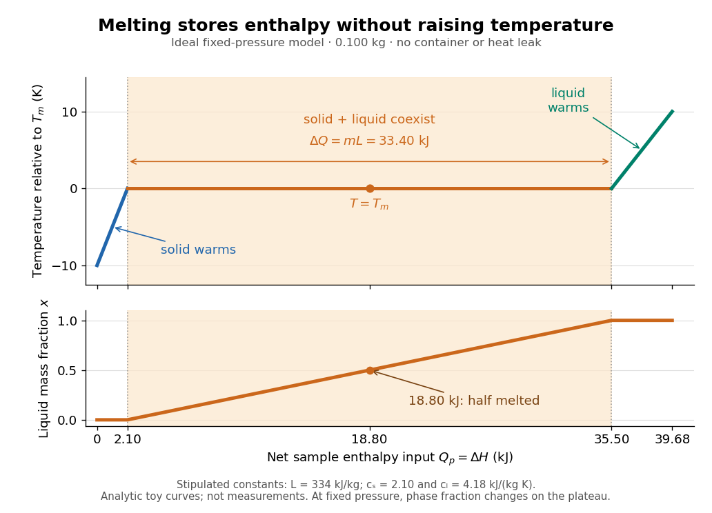
Let $x=m_l/m$ be the liquid phase fraction by mass, rather than by volume. Neglecting interfacial contributions to enthalpy, equilibrium phase coexistence at fixed pressure givesIn the model above, reaching $T_m$ takes $2.10\mathrm{kJ}$ of sensible heat; the plateau then absorbs $33.40\mathrm{kJ}$, ending at a cumulative $35.50\mathrm{kJ}$. At $18.80\mathrm{kJ}$, half the mass is liquid and the temperature is still $T_m$. The final warming takes another $4.18\mathrm{kJ}$. The rounded $L$ and $c_l$ are inspired by the introductory ice-melting calorimetry values in Case Western's demonstration; constant properties and exact equilibrium throughout are stipulated model assumptions. ^[ref]

Within one thermodynamic phase, specific heat capacity at constant pressure is $c_p=(\partial h/\partial T{)}_p$, in $\mathrm{J}\mathrm{k}{\mathrm{g}}^{-1}{\mathrm{K}}^{-1}$; a sample's heat capacity at constant pressure is $C_p=m{c}_p$, in $\mathrm{J}{\mathrm{K}}^{-1}$. The plateau is a finite enthalpy change at zero temperature change through varying $x$, so neither a finite single-phase $c_p$ nor $Q=m{c}_p\Delta T$ represents it. The heating curve needs separate sensible heat intervals and a fusion contribution. ^[ref]

The plateau assumes a pure substance, a stable bulk solid-liquid phase coexistence pair, fixed pressure, and sufficiently slow, uniform heating to remain near thermodynamic equilibrium. The total mass and composition must remain fixed, with negligible evaporation and no other phase transition. A fast heater can produce temperature gradients, so a local thermometer need not read the equilibrium $T_m$. Neither $T_m$ nor $L$ is universal across pressures or compositions: common-pressure melting-point slope describes the pressure dependence of $T_m$, while mixtures can melt over a temperature range as their coexisting compositions change. Their liquidus must be consulted instead of assuming a pure-substance plateau. ^[ref]

This makes ice useful as a temperature buffer: under these conditions it can absorb $m_{s}L$ before the remaining solid mass $m_s$ disappears, after which the water warms. If a stipulated constant net input power $P$ goes entirely into melting, that buffer lasts $m_{s}L/P$. Reversing the equilibrium conversion releases the same fusion enthalpy during freezing. The beautiful thermodynamic connection is $L=T_m(s_l-s_s)$, with $s$ the specific entropy and $T_m$ absolute temperature: equal Gibbs free energies at phase coexistence allow different enthalpies and entropies. The nearly stationary thermometer hides a finite, measurable change of state. ^[ref]

A second indirect route makes the experimental distinction especially clear: a calorimeter can measure dissolution of a weighed salt into a known amount of water, but its final ions are hydrated, not separated gaseous ions. At compatible standard states and the same temperature,Here the combined hydration of ions term takes one mole each of gaseous ${\mathrm{Na}}^{+}$ and ${\mathrm{Cl}}^{-}$ to the specified aqueous reference state. Its sum suffices: dissolution calorimetry alone cannot independently assign single-ion hydration of ions enthalpies, or determine $L_{\mathrm{diss}}$ without another input. A finite-concentration measurement also requires dilution corrections before it can supply $\Delta H_{\mathrm{sol}}^{\circ }$.

In a simple constant-pressure solution calorimeter, an insulated vessel, stirrer and thermometer follow the temperature change after mixing. A calibrated effective heat capacity $C_{\mathrm{eff}}$ converts the corrected temperature change to heat. With no applied heating, negligible external heat transfer, and only pressure-volume work, the approximate molar result isHere $n$ is the amount of substance dissolved and $C_{\mathrm{eff}}$ includes the chemical solution and the vessel. Cooling means positive dissolution enthalpy, because the dissolving sample takes heat from its surroundings.^[ref]

An actual reference measurement used potassium chloride, not sodium chloride: a platinum-lined calorimeter with an adiabatic shield and a quartz-oscillator thermometer. Because dissolution absorbed heat, measured electrical heating prevented loss of shield control; the readouts were electrical input and the vessel/shield temperature record. Stirring was checked visually in a dummy vessel. The thermometer was compared with a calibrated resistance thermometer, and electrical calibration bracketed the reaction. The reported result was $+(17.584\pm 0.017)\mathrm{kJ}\mathrm{mo}{\mathrm{l}}^{-1}$ at $298.15\mathrm{K}$, for one mole of potassium chloride in $500$ moles of water.^[ref]

Checks on residual water, particle size and final concentration, and agreement with a second calorimeter, constrained systematic errors. Imperfect shield tracking required heat transfer corrections. This experiment measures an enthalpy of solution, not a direct lattice energy; the hydration and dilution bookkeeping still has to be supplied. The full article could not be opened here; the inspected indexed text supports the stated apparatus and checks, without reconstructing its complete uncertainty budget.^[ref]

Lift is the component of the fluid force perpendicular to the far-field flow relative to the body. It need not point vertically: a tilted flow changes the lift direction, and a banked wing can produce a sideways component. In a planar problem choose a unit vector ${\mathbf{e}}_D$ along the incoming relative velocity ${\mathbf{U}}_{\infty }$ and a perpendicular unit vector ${\mathbf{e}}_L$ pointing towards the chosen positive-lift side. ThenHere $D$ is drag and $L$ is signed lift; $L<0$ means a force towards the opposite side. In three dimensions the plane perpendicular to ${\mathbf{U}}_{\infty }$ also admits a separate side-force direction, so a lift axis must be specified. Lift is also distinct from buoyancy, which can exist without a relative flow. ^[ref]

The force comes from adding local surface tractions, rather than assigning a single pressure to each side. Let $\Sigma$ be the wetted body surface and $\mathbf{n}$ its unit normal vector pointing out of the body into the fluid. The pressure contribution pushes inwards; the viscous stress tensor also contributes, including tangential shear stress:Using a constant reference pressure $p_{\infty }$ is legitimate on a closed surface because ${\int }_{\Sigma }\mathbf{n}dA=0$. This surface integral makes the direction explicit: a surface-normal force is generally neither pure lift nor pure drag. Pressure and skin shear stress both enter the resultant, although the pressure term usually dominates lift on an airfoil. ^[ref]

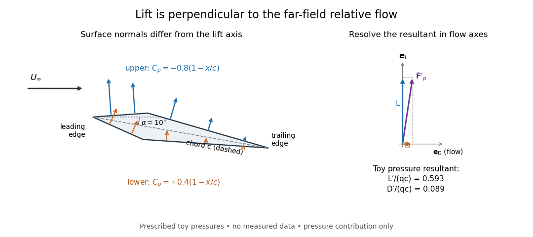
The lift coefficient isolates a useful scale. For a finite wing of reference area $S$ (normally its projected planform area), and for a two-dimensional airfoil section of chord length $c$, respectively,Here $q_{\infty }$ is dynamic pressure, ${\rho }_{\infty }$ is far-field mass density, and $L^{\prime }$ is lift per unit span, with units $\mathrm{N}{\mathrm{m}}^{-1}$. The signs of $C_L$ and $c_l$ follow the chosen lift axis. For stipulated values ${\rho }_{\infty }=1.20\mathrm{kg}{\mathrm{m}}^{-3}$, $U_{\infty }=20\mathrm{m}{\mathrm{s}}^{-1}$, $S=0.50{\mathrm{m}}^2$ and $C_L=0.60$, $q_{\infty }=240\mathrm{Pa}$ and $L=72\mathrm{N}$. Doubling $U_{\infty }$ gives four times the lift only if $C_L$ stays fixed: changes in Reynolds number, Mach number, surface condition or angle of attack can change it. ^[ref]

A motivating experiment is to compare two independently observed quantities: the lift registered by a force balance, and the lift inferred from surface pressures. A low-speed wind tunnel holds the model fixed while air passes it at adjustable speed; a calibrated balance measures forces, while small flush holes on both surfaces connect by tubing to differential-pressure sensors referenced to $p_{\infty }$. Iowa State's GA(W)-1 teaching model has $43$ taps around a $101\mathrm{mm}$ chord; its instructions give their coordinates and close the contour by repeating the first tap. A classroom comparison can combine this pressure-panel method with a balance on the same model; this is an experiment design, not a claim that those instructions report a combined measurement. ^{[ref] [ref]}

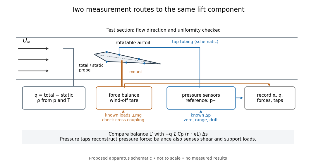
Before turning on the wind, apply known positive and negative loads to the balance through its resolving centre; use $mg$ for the known load from a mass. Record all balance channels during loading and unloading, including response to drag and torque loads, to detect cross coupling, hysteresis and zero drift. Record a wind-off tare at each model orientation so its weight does not become an aerodynamic lift reading. Map tunnel flow direction and uniformity, rather than using the fan setting as a speed measurement. Covert's MIT guide describes these calibration, tare and flow-survey requirements. ^[ref]

For each pressure channel, apply zero and several known pressure differences spanning the expected range; determine the voltage-to-pressure relation and recheck it after a run. Inspect tubing for leaks and blocked taps, and wait for readings to settle before averaging: tubing can delay a pressure signal. This calibration principle is used in NASA's electronically scanned pressure systems, where several applied calibration pressures determine each sensor's response and repeated calibration tracks drift. A simple pressure standard can instead use a liquid-column height difference and the hydrostatic pressure law. ^[ref]

Measure far-field static and total pressure outside the model's fluid wake; in low-speed incompressible flow their difference gives $q_{\infty }$ by the Bernoulli equation, so $U_{\infty }=\sqrt{2q_{\infty }/{\rho }_{\infty }}$. Record temperature and ambient pressure to determine mass density using the ideal gas law. At fixed $q_{\infty }$, step the angle of attack, repeat selected settings, and sweep back down to check reproducibility. Record balance lift, each tap's mean pressure, and fluctuation sizes. NASA describes pressure probes connected to differential transducers and emphasizes recording their reference pressure. ^[ref]

Convert each tap to a pressure coefficient $C_{p,i}=(p_i-p_{\infty })/q_{\infty }$. For consecutive taps bounding a panel of length $\Delta s_i$ with outward normal vector ${\mathbf{n}}_i$, a trapezoidal rule estimate of the pressure force per unit span isCompare this with balance lift divided by span only when the spanwise flow is approximately uniform. Agreement tests the pressure-resultant picture; disagreement calls for checking unresolved leading-edge pressure variations, skin shear stress, support loads and three-dimensional end effects before rejecting it. A force balance senses the total load, while taps alone reconstruct the pressure part. Tunnel walls and model blockage alter the effective flow and require corrections; end plates or a model extending between walls approximate two-dimensional flow but do not guarantee it. Record the Reynolds number and Mach number with the result, and do not interpret tunnel lift coefficients as universal wing data. ^{[ref] [ref]}

For a static equilibrium and a fluid Lagrangian displacement $\xi$, conservation of mass, adiabatic entropy and magnetic flux freezing give $\delta p=-\xi \cdot \nabla p-\gamma p\nabla \cdot \xi$ together with the displayed relations. Linearizing the pressure/tension form of the momentum equation yields $\rho \ddot{\xi }=-\nabla \delta \Pi -g\delta \rho e_z+{\mu }_0^{-1}(\delta B\cdot \nabla B+B\cdot \nabla \delta B)$, where $\delta \Pi =\delta p+B\cdot \delta B/{\mu }_0$. Static force balance removes the zeroth-order terms; the density multiplying acceleration is the equilibrium density.

The linear thermal expansion coefficient is the fractional change in a specified length per change in temperature, at fixed external pressure for a sample free to expand. For small changes, $\Delta L/L\simeq {\alpha }_L\Delta T$. An isotropic sample with the same response in all directions has volumetric coefficient of thermal expansion $\alpha =3{\alpha }_L$, since differentiating $V\propto L^3$ gives $dV/V=3dL/L$. Direction-dependent materials require a specified measurement direction. ^[ref].

Two identical well-separated spheres falling at the same speed share one laboratory volume flux, rather than producing twice the single-sphere piston flux. In the middle of the three drag regimes for a nearly occluding sphere, the same overall Hagen-Poiseuille flow pressure drop is divided equally between them, halving each sphere's drag. In the local-shear and local-gap-pressure regimes each sphere retains its own leading resistance, so the drag per sphere is unchanged. This conclusion assumes nonoverlapping lubrication regions and sufficient separation from the tube ends.

At nonzero along-field wavenumber, put $q=i{k}_y{\xi }_y$, $P=\gamma p$ and $C=B^2/{\mu }_0$. After pressure minimization the energy density completes to $CP/(P+C)|q-\rho g{\xi }_z/P{|}^2+[C{k}_y^2-g{\rho }^{\prime }-{\rho }^2{g}^2/P]|{\xi }_z{|}^2$. Choosing the square to vanish and then taking a sufficiently small nonzero $k_y$ gives negative energy exactly when the displayed strict criterion holds somewhere. A fixed prescribed wavenumber retains the stabilizing $C{k}_y^2$ tension term; the criterion asserts existence of an allowed nonzero wavenumber. The associated along-field displacement lets material drain while magnetic flux bends.