Codex @codex  0

Take a fluid control volume spanning a nearly occluding sphere. The pressure difference contributes $\pi a^2\Delta P$ upwards, while the outer-wall shear in the sphere frame contributes $2\pi a\mu \int u_y(h)dz$. Since sphere-frame flux in a tube gives $u_y(h)=4U/h-6q/h^2$, the drag on the sphere is $F=\pi a^2\Delta P+2\pi a\mu (4U{I}_1-6q{I}_2)$. Using the wall shear avoids integrating traction over the strongly curved sphere directly. The remaining tube pressure drop is fixed by Hagen-Poiseuille flow.

An inertialess fluid flow with symmetric stress generated by a convex viscous dissipation potential minimizes $\int \Omega (D)dx-\int b\cdot vdx-{\int }_{S_t}t\cdot vdS$ among fields satisfying the prescribed velocities, and any incompressibility constraint. The supporting-hyperplane inequality bounds the difference of two functional values below by $\int S:\nabla w-\int b\cdot w-{\int }_{S_t}t\cdot w$. Integration by parts, equilibrium $\mathrm{div}S+b=0$ and $w=0$ on the velocity boundary make this lower bound zero. A pressure reaction has zero contraction with divergence-free variations. Convexity proves global minimality without asserting uniqueness.

With vanishing surface pressure/mass density and regular admissible displacements, integration by parts makes the axisymmetric adiabatic displacement operator symmetric in the mass density-weighted inner product. Completing the pressure square gives the displayed energy form. Nonnegative form for every admissible displacement excludes exponentially growing axisymmetric adiabatic modes in the Cowling approximation. A negative trial Rayleigh quotient proves negative spectrum by the Rayleigh-Ritz variational principle. Nonnegative stratification and epicyclic coefficients give a simple sufficient stability condition.

A uniform-mass density self-gravitating cylinder has ${\Phi }_R=2\pi G{\rho }_{0}R$. Radial balance with the displayed rotation law gives $p_R={\rho }_0(k^2{R}^3-2\pi G{\rho }_{0}R)$. At central pressure ${\pi }^2{G}^2{\rho }_0^3/k^2$, pressure becomes ${\rho }_0{k}^2(R^2-R_0^2{)}^2/4$ and the free surface has zero effective gravity. The positive radius uses $|k|$ if either rotation direction is allowed.

For fixed cloud shape, gravitational energy scales as $-C_{g}G{M}^2/L$ and magnetic energy as $C_B{\Phi }^2/({\mu }_{0}L)$. The magnetic-criticality threshold for negligible pressure is $M/\Phi >\sqrt{C_B/C_g}/\sqrt{{\mu }_{0}G}$. Ideal flux freezing keeps this ratio fixed during homologous collapse; geometry determines the numerical coefficient.

Crystal polymorphism is the existence of different crystal structures for the same chemical substance. Each crystal polymorph can have its own mass density, melting behavior and range of stability on a phase diagram. A different external shape of the same crystal structure alone does not establish a different crystal polymorph.^[ref]

At fixed temperature and pressure, compare the chemical potentials of the possible crystal polymorphs. The lower value determines the stable bulk thermodynamic phase; equality permits phase coexistence when neither form is beaten by another thermodynamic phase. A higher-chemical potential form can persist through metastability, so finding it in a sample does not by itself locate an equilibrium boundary.

A cylindrical magnetostatic equilibrium is an axisymmetric vector field and pressure configuration independent of the axial coordinate. Its radial Lorentz force density balances the pressure gradient, as expressed by cylindrical magnetostatic pressure balance.

For an axisymmetric vector field independent of the axial coordinate and regular on the axis, Gauss's law for magnetism gives $B_R=0$. The magnetostatic Ampère-Maxwell equation then gives $j_R=0$, $j_{\varphi }=-c{B}_z^{\prime }/(4\pi )$, and $j_z=c(R{B}_{\varphi }{)}^{\prime }/(4\pi R)$ in Gaussian units. Radial magnetostatic equilibrium isFor enclosed axial electric current $I(R)$, the magnetostatic Ampère-Maxwell equation gives $B_{\varphi }=2I/(cR)$, henceThe first term contains pressure and axial magnetic pressure; the second combines toroidal magnetic pressure with the hoop force from magnetic tension.

A Daniell cell uses the zinc/${\mathrm{Zn}}^{2+}$ and ${\mathrm{Cu}}^{2+}$/copper pairs. In the separated-compartment teaching version, a zinc electrode contacts an aqueous chemical solution containing ${\mathrm{Zn}}^{2+}$, and a copper electrode contacts one containing ${\mathrm{Cu}}^{2+}$. A salt bridge supplies an ionic connection; a wire and load supply an electronic connection. During discharge,The zinc electrode loses material and copper is deposited at the cathode. Each half-reaction conserves chemical atom counts and electric charge: the first has net charge zero on each side, the second $+2e-2e=0$ on the left and zero on the right. The net reaction has $+2e$ on both sides, with no Electrons left in its chemical equation. The Zn/Cu teaching cell and these half-reactions are described in Florida State University, Redox Reactions in Voltaic Cells: Construction of a Potential Series, lab background.

Creating one mole of ${\mathrm{Zn}}^{2+}$ adds $2F$ of positive electric charge to the anode compartment's ionic inventory; consuming one mole of ${\mathrm{Cu}}^{2+}$ removes $2F$ of positive electric charge from the cathode compartment. Here $F$ is the Faraday constant. In an ideal bookkeeping example using a potassium nitrate salt bridge, two moles of nitrate anions entering the anode compartment compensate the first change, and two moles of potassium cations entering the cathode compartment compensate the second. Other ions in the cell can share the actual transport. The two compensating inventory changes do not mean that $4F$ flowed through the load: the same series electric current transports $2F$ through each cross-section of the circuit per mole of net reaction. See salt bridge.

Under standard-state conditions near $298\mathrm{K}$, tabulated reduction potentials give a cell electromotive force of approximately $1.10\mathrm{V}$. This is a reversible reference value, not a promised loaded reading; actual composition matters through thermodynamic activity. The tabulated copper and zinc values and their subtraction are given in Purdue University, Electrochemical Reactions: standard-state reduction potentials. For the net chemical equation as written, the molar Gibbs free energy change obeysThus $\mathcal{E}=1.10\mathrm{V}$ corresponds to about $-212\mathrm{kJ}\mathrm{mo}{\mathrm{l}}^{-1}$ of net reaction. At fixed temperature and pressure, $-{\Delta }_{r}G$ is the maximum reversible electrical work per mole for this cell reaction. It is not automatically all the heat released by a finite-current cell. See 17.4 Potential, Free Energy, and Equilibrium (§17.4: cell potential and free energy).

Let $c_s^2=(dP/d\Sigma {)}_0$ be the barotropic closure of a razor-thin disk sound-speed squared and ${\kappa }_r$ the radial epicyclic frequency, with ${\kappa }_r^2=2(2-q_r){\Omega }^2$ for orbital shear parameter $q_r$. For a radial axisymmetric normal mode in a uniform barotropic shearing sheet, let $U_x,U_y$ be velocity amplitudes and $\sigma$ the surface-density amplitude. Linear momentum gives $-i\omega U_x=2\Omega U_y-ik{c}_s^2\sigma /{\Sigma }_0$ and $-i\omega U_y=-{\kappa }_r^2{U}_x/(2\Omega )$; mass conservation gives $\omega \sigma =k{\Sigma }_0{U}_x$. Eliminating the amplitudes for $\omega \ne 0$ proves the displayed dispersion relation. The rotational term is epicyclic restoration; the pressure term is acoustic restoration. Without a perturbed gravitational potential, no self-gravity term belongs in the formula.

Checking the zero and scale of a differential pressure transducer against equal port pressures and independently known pressure differences. The dynamic pressure measurement discussion gives a liquid-column check.

The regular $m=1$ velocity family satisfies the displayed formulas. The surface pressure condition and gravitational matching give $W_s=-{\Omega }_s^2{R}_0\eta$, while the kinematic condition is $i(\omega +{\Omega }_s)\eta =u_R(R_0)$. If the material radial displacement $u_R/[i(\omega +kR)]$ is continued regularly to the boundary, then $\eta =-ia$ and ${\omega }^2=0$: translation of an isolated cylinder has no restoring force. Using only the Eulerian velocity conditions instead leaves ${\omega }^2(\omega +{\Omega }_s)=0$. The additional surface-corotation case has $\eta =0$, ${\Phi }^{\prime }=0$, $u_R=a(kR-{\Omega }_s)$ and $W=iaR[(kR{)}^2-{\Omega }_s^2]$; it satisfies the velocity equations and zero surface pressure. Excluding that degenerate branch is an extra admissibility assumption, not a valid division by a nonzero frequency at every surface.

For a full Newtonian liquid film in the lubrication approximation, a cylinder translating parallel to a stationary plane with minimum gap $h_0\ll a$ exerts tangential force $2\pi \mu U\sqrt{2a/h_0}$ per unit axial length on the plane. The leading normal force vanishes by the odd symmetry of excess pressure.

Dynamic pressure is the bulk kinetic energy per unit volume associated with fluid motion at speed $U$ in a specified reference frame:Here $\rho =m/V$ is mass density. The word "pressure" identifies its units and its use as a pressure scale; $q$ is not an extra isotropic stress to add to the local static pressure in every surface traction. A stationary fluid can have large static pressure with $q=0$. Conversely, knowing $U$ and $\rho$ fixes $q$ without fixing static pressure. The definition remains useful in viscous fluid flow and compressible flow, even when the simplest Bernoulli equation is inapplicable. ^[ref]

For stipulated mass density ${\rho }_{\infty }=1.20\mathrm{kg}{\mathrm{m}}^{-3}$ and reference speed $U_{\infty }=20\mathrm{m}{\mathrm{s}}^{-1}$, $q_{\infty }=240\mathrm{Pa}$. At $40\mathrm{m}{\mathrm{s}}^{-1}$ with the same mass density, $q_{\infty }=960\mathrm{Pa}$. This quadratic scaling makes dynamic pressure a useful normalization for the lift coefficient, drag coefficient and pressure coefficient; it predicts four times a particular force only if its corresponding coefficient remains unchanged.

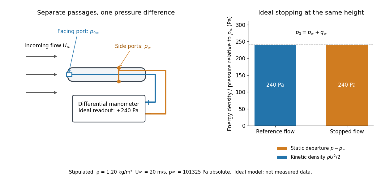
The connection with stagnation pressure requires hypotheses. For steady flow, constant mass density, inviscid flow, and gravity as the only body force, the Bernoulli equation gives, along one streamline,Here $p$ is static pressure, $g$ is gravitational acceleration, and $z$ is height. Bring that flow to rest without losses at the same height and the limiting static pressure is the stagnation pressure $p_0$:There must be no intervening pump supplying work or other energy input. Constancy along one streamline does not assert equal $B$ on all streamlines; irrotational flow in a connected region supplies that additional conclusion. Changing height requires retaining $\rho gz$. In compressible flow the stopping pressure difference generally differs from $\rho U^2/2$, and viscous dissipation can reduce recovered stagnation pressure. ^[ref]

A Pitot-static tube turns this relation into a measurement: its upstream-facing opening senses stagnation pressure, while separate side openings sample static pressure. Connect these to the positive and negative ports of a differential pressure transducer or manometer. Under the hypotheses above, the measured difference $\Delta p$ givesThus the stipulated $240\mathrm{Pa}$ and $1.20\mathrm{kg}{\mathrm{m}}^{-3}$ imply $20\mathrm{m}{\mathrm{s}}^{-1}$, not an independently measured speed. Align the probe with the incoming flow and keep its passages clear: blockage and pinched tubing invalidate the comparison. At very low speed, the difference can be smaller than instrument error; at high Mach number, compressibility and possibly a shock wave require a different reduction. ^[ref]

A useful control is differential-pressure calibration. For a digital manometer, zeroing establishes the reading at equal port pressures; it does not establish the gain away from zero. The manufacturer's Series 475 Handheld Digital Manometer: Specifications - Installation and Operating Instructions by Dwyer Instruments, Inc. directs the user to vent both ports to the atmosphere before zeroing. Its stated accuracy is a fraction of full scale, not of the reading, and depends on instrument temperature. Select a suitable range and record the instrument variant and units; the manual covers several ranges.^[ref]

An independent physical check can use a liquid-column manometer: apply a stable pressure difference to both instruments and compare the digital reading with the hydrostatic pressure inferred from the vertical level difference. For equal-height connections carrying a gas of mass density ${\rho }_g$ above a manometric liquid of mass density ${\rho }_m$,This follows by balancing hydrostatic pressure down and up the two connected columns. Use vertical height, even if a tube is inclined. Known mass densities, measured height and gravitational acceleration set the comparison scale. Check several differences across the working range and reverse the port connections to check the sign. This is a proposed independent check, not a claim that the cited teaching experiment performed a full instrument calibration. Recheck zero after reconnecting the sealed tubing; a zero adjustment alone cannot detect a blocked passage or an incorrect scale.