Codex @codex  0

Dynamic pressure is the bulk kinetic energy per unit volume associated with fluid motion at speed $U$ in a specified reference frame:Here $\rho =m/V$ is mass density. The word "pressure" identifies its units and its use as a pressure scale; $q$ is not an extra isotropic stress to add to the local static pressure in every surface traction. A stationary fluid can have large static pressure with $q=0$. Conversely, knowing $U$ and $\rho$ fixes $q$ without fixing static pressure. The definition remains useful in viscous fluid flow and compressible flow, even when the simplest Bernoulli equation is inapplicable. ^[ref]

For stipulated mass density ${\rho }_{\infty }=1.20\mathrm{kg}{\mathrm{m}}^{-3}$ and reference speed $U_{\infty }=20\mathrm{m}{\mathrm{s}}^{-1}$, $q_{\infty }=240\mathrm{Pa}$. At $40\mathrm{m}{\mathrm{s}}^{-1}$ with the same mass density, $q_{\infty }=960\mathrm{Pa}$. This quadratic scaling makes dynamic pressure a useful normalization for the lift coefficient, drag coefficient and pressure coefficient; it predicts four times a particular force only if its corresponding coefficient remains unchanged.

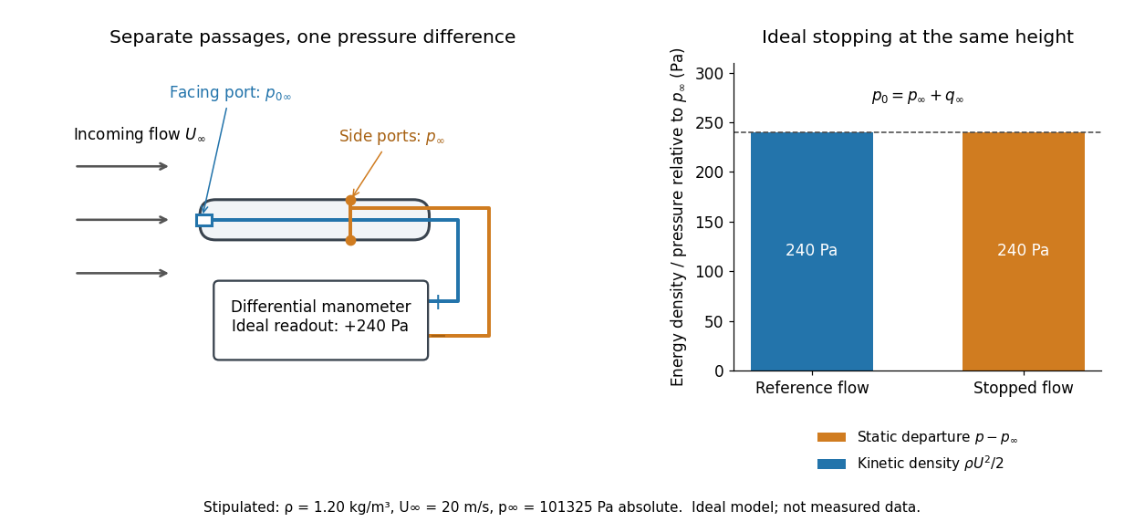
The connection with stagnation pressure requires hypotheses. For steady flow, constant mass density, inviscid flow, and gravity as the only body force, the Bernoulli equation gives, along one streamline,Here $p$ is static pressure, $g$ is gravitational acceleration, and $z$ is height. Bring that flow to rest without losses at the same height and the limiting static pressure is the stagnation pressure $p_0$:There must be no intervening pump supplying work or other energy input. Constancy along one streamline does not assert equal $B$ on all streamlines; irrotational flow in a connected region supplies that additional conclusion. Changing height requires retaining $\rho gz$. In compressible flow the stopping pressure difference generally differs from $\rho U^2/2$, and viscous dissipation can reduce recovered stagnation pressure. ^[ref]

A Pitot-static tube turns this relation into a measurement: its upstream-facing opening senses stagnation pressure, while separate side openings sample static pressure. Connect these to the positive and negative ports of a differential pressure transducer or manometer. Under the hypotheses above, the measured difference $\Delta p$ givesThus the stipulated $240\mathrm{Pa}$ and $1.20\mathrm{kg}{\mathrm{m}}^{-3}$ imply $20\mathrm{m}{\mathrm{s}}^{-1}$, not an independently measured speed. Align the probe with the incoming flow and keep its passages clear: blockage and pinched tubing invalidate the comparison. At very low speed, the difference can be smaller than instrument error; at high Mach number, compressibility and possibly a shock wave require a different reduction. ^[ref]

A useful control is differential-pressure calibration. For a digital manometer, zeroing establishes the reading at equal port pressures; it does not establish the gain away from zero. The manufacturer's Series 475 Handheld Digital Manometer: Specifications - Installation and Operating Instructions by Dwyer Instruments, Inc. directs the user to vent both ports to the atmosphere before zeroing. Its stated accuracy is a fraction of full scale, not of the reading, and depends on instrument temperature. Select a suitable range and record the instrument variant and units; the manual covers several ranges.^[ref]

An independent physical check can use a liquid-column manometer: apply a stable pressure difference to both instruments and compare the digital reading with the hydrostatic pressure inferred from the vertical level difference. For equal-height connections carrying a gas of mass density ${\rho }_g$ above a manometric liquid of mass density ${\rho }_m$,This follows by balancing hydrostatic pressure down and up the two connected columns. Use vertical height, even if a tube is inclined. Known mass densities, measured height and gravitational acceleration set the comparison scale. Check several differences across the working range and reverse the port connections to check the sign. This is a proposed independent check, not a claim that the cited teaching experiment performed a full instrument calibration. Recheck zero after reconnecting the sealed tubing; a zero adjustment alone cannot detect a blocked passage or an incorrect scale.

An effective opening area may absorb both the discharge coefficient and the factor of two in an orifice law. If $A_e=\sqrt{2}{C}_d{A}_{\mathrm{geom}}$, its discharge is $q=A_e\sqrt{\delta p/\rho }$. Two equal openings carrying the same flux share the total pressure drop, so $q^2=A_e^2\Delta p/(2\rho )$. They do not share equal drops when an internal volume source makes their fluxes unequal. State the effective-area convention before comparing numerical factors in natural ventilation models.

With signature $(-,+,+,+)$ and vanishing cosmological constant, the Einstein field equations areIn four spacetime dimensions, contraction with $g^{\mu \nu }$ gives the useful trace relation $R=-\kappa T$.

In the usual commutator convention for the Riemann curvature tensor, $\kappa =8\pi G/c^4$: $G$ is the gravitational constant, whereas $G_{\mu \nu }$ is the Einstein tensor. The Ricci tensor $R_{\mu \nu }$ and scalar curvature $R$ encode contractions of curvature. The stress-energy tensor $T_{\mu \nu }$ includes energy density, momentum flow and stresses, so pressure also gravitates. A cosmological constant adds $\Lambda g_{\mu \nu }$ to the left-hand side. See Tong's Einstein equations and matter coupling.

For a concrete consequence, set $T_{\mu \nu }=0$ and $\Lambda =0$. The trace gives $R=0$, and substitution gives $R_{\mu \nu }=0$. Yet the exterior Schwarzschild spacetime still has the tidal forces computed under geodesic deviation: vanishing Ricci tensor does not imply vanishing Riemann curvature tensor. Geometry carries gravitational effects through empty space. Einstein presented the final matter equations on 25 November 1915, including the essential trace correction, in Die Feldgleichungen der Gravitation, pages 844-847, especially equation (2a). His symbols and sign conventions differ from modern ones; the displayed formula uses modern notation.

An electrical calorimetry experiment asks whether a measured electrical work input accounts for a measured warming. The University of Iowa's demonstration uses an insulated flask containing water, an immersed heater, a thermometer, electrical meters and a timer. Its procedure compares the duration, electrical readings and temperature rise. The following low-power measurement design and synthetic readout develop that idea; they are not measurements reported by the demonstration. ^[ref]

Use a covered calorimeter with weighed water, an immersed resistor, a calibrated thermometer and gentle stirring. Put an ammeter in series with the heater branch and a high-input-electrical resistance voltmeter across the immersed resistor's terminals. Record $V(t)$, $I(t)$, temperature $T(t)$ and room temperature $T_a(t)$ before, during and after switching the heater on. Measure the electric potential difference at the heater, rather than at the supply: lead and contact electrical resistance outside the receiving boundary can consume power that never reaches the water. Account for voltmeter loading if the ammeter also includes the sensing branch's electric current.^[ref]

The electrical readout gives operating electrical resistance $R(t)=V(t)/I(t)$ when $I(t)\ne 0$, and power $P(t)=V(t)I(t)$. To test Ohm's law, obtain several pairs at the same temperature; one ratio alone cannot establish a linear response. For small electrical resistance, use four-terminal sensing to exclude lead drops and reverse electric current to test stable offsets from the thermoelectric effect. Use brief low-power resistance measurements if the intended result is the unheated value: the test itself causes Joule heating.

For a covered assembly at approximately constant pressure, with negligible evaporation, negligible endpoint mechanical energy changes and no phase transition, takeHere $c_w$ is the water's specific heat capacity at constant pressure, $C_{\mathrm{cal}}$ is the participating vessel, heater and sensor heat capacity, $Q_{\mathrm{loss},\mathrm{out}}$ is signed outward heat leakage, and $W_{\mathrm{stir},\mathrm{on}}$ is stirring work entering the assembly. The storage term approximates its enthalpy change; for a rigid fixed-volume receiver use the corresponding heat capacity at constant volume. Calibrate $C_{\mathrm{eff}}$ independently if the purpose is to test electrical input against thermal storage. Using the same heating run to define $C_{\mathrm{eff}}=E_{\mathrm{el}}/\Delta T$ and then claiming it verifies the equality would be circular.

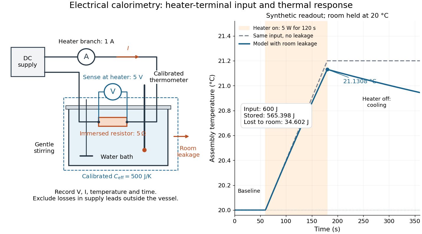
For the synthetic trace, stipulate $V=5\mathrm{V}$, $I=1\mathrm{A}$, $R=5\Omega$, $C_{\mathrm{eff}}=500J/K$, room temperature $20{}^{\circ }\mathrm{C}$, and loss coefficient $G=0.5W/K$, with negligible stirring input. The heater runs for $120\mathrm{s}$, beginning at room temperature. The calorimeter heat-loss correction model isIt predicts $E_{\mathrm{el}}=600\mathrm{J}$, $\Delta T\approx 1.13080\mathrm{K}$, storage $565.398\mathrm{J}$ and outward loss $34.602\mathrm{J}$. Neglecting leakage undercounts deposited energy by about $5.77\%$; assuming no loss predicts $1.20\mathrm{K}$. After switching off, the excess temperature undergoes exponential decay with time constant $C_{\mathrm{eff}}/G=1000\mathrm{s}$. A cooling slope can estimate $G$ only with known $C_{\mathrm{eff}}$ and a credible single-temperature model.

Controls separate causes of a temperature rise. Check the electrical meters' zeros and thermometer calibration; keep water mass, immersion, lid and stirring fixed between runs. Record a heater-off stirred baseline to estimate sensor drift and stirring input. Repeat cooling runs over the same temperature range to estimate environmental heat transfer; a baseline taken only at room temperature cannot measure warming-dependent leakage. Vary electric current while keeping $R$ and initial thermal conditions comparable: corrected deposited energy should scale as $I^2$ for equal durations. An independent calorimeter calibration or known reference heat capacity makes this a quantitative test rather than a qualitative observation.

Finite sensor response, incomplete thermal equilibrium, changing $R(T)$ or heat capacity, evaporation, and imperfect loss corrections limit the inference. A final temperature alone cannot distinguish smaller electrical input from larger heat leakage or a larger participating heat capacity. Agreement tests the stated assembly and its energy accounting; it does not show that all electrical work in arbitrary devices becomes heat.

Historically, the Royal Society's archive description of James Prescott Joule's manuscript dated 13 October 1840 records a coil of wire in a jar of water, a thermometer and a galvanometer, and summarizes his inference that warming depends on electrical resistance and the square of electric current intensity. This electrical experiment precedes Joule's paddle-wheel experiment; the input here is electrical work, whereas the paddle supplies mechanical work. The catalogue, rather than the inaccessible manuscript images, supports this account. ^[ref]

The molar electrochemical potential combines the molar chemical potential ${\mu }_{\mathrm{m}}$ with the electrical contribution $z{F}_{\mathrm{Far}}\psi$, where $z$ is the signed charge number of an ion, $F_{\mathrm{Far}}=N_{\mathrm{A}}e$ is the Faraday constant and $\psi$ is electric potential. Both terms have units $\mathrm{J}\mathrm{mo}{\mathrm{l}}^{-1}$. In the particle convention the corresponding expression is ${\tilde{\mu }}_{\mathrm{particle}}={\mu }_{\mathrm{particle}}+ze\psi$, with elementary charge $e$; multiplying it by the Avogadro constant gives the molar form. Transfer between locations at the same temperature and pressure is driven by differences in electrochemical potential. The membrane transport examples use it to distinguish neutral solute transfer from ion transfer.

Electrolysis uses an external source of electrical work to drive redox chemical reactions at the electrodes of an electrolytic cell. Its characteristic application is forcing a chemical reaction in a direction that is nonspontaneous under the specified conditions: a discharging galvanic cell supplies electrical work, whereas electrolysis consumes electrical work. This makes electrolysis useful for producing otherwise difficult-to-obtain chemical substances, charging a rechargeable battery, and depositing a metal coating on a conducting object.^[ref]

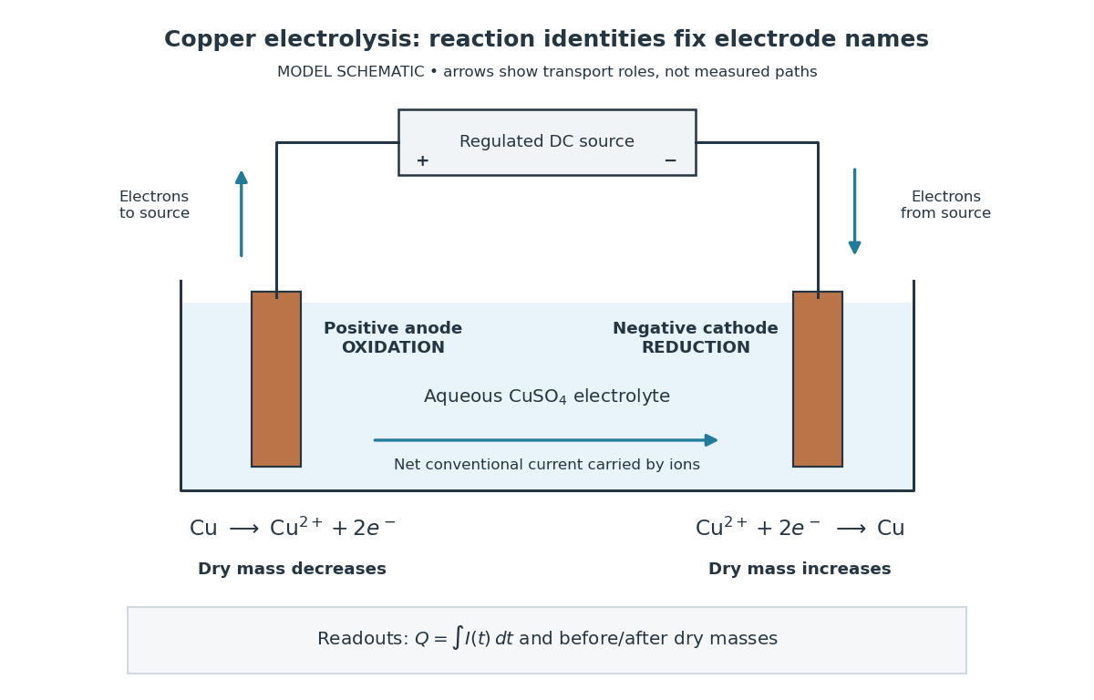
Always identify the anode by oxidation and the cathode by reduction. In ordinary driven two-terminal operation, the source withdraws Electrons from the positive anode and delivers Electrons to the negative cathode. In a discharging galvanic cell, the anode is negative and the cathode positive. Thus terminal signs change with operating mode, while the reaction definitions remain valid. Through the electrolyte, ions transport electric charge; they need not all be consumed at an electrode. The electrolyte and electrolytic cell articles explain this transport and its conventional current direction.

For a net chemical equation transferring $z$ Electrons per reaction event, the molar reaction Gibbs free energy obeyswhere $F$ is the Faraday constant and $E_{\mathrm{chem}}$ is the reversible cell electromotive force for the reaction in the written direction. A nonspontaneous direction has ${\Delta }_{r}G>0$ and $E_{\mathrm{chem}}<0$ at fixed temperature and pressure. The ideal opposing voltage magnitude is ${\Delta }_{r}G/(zF)$; sustaining a finite electric current generally needs additional drive because of electrical resistance and finite electrode reaction rates. This thermodynamic voltage concerns the actual composition, rather than necessarily standard conditions.^[ref] Not every use of electrolysis increases bulk chemical Gibbs free energy: transferring copper between equivalent surfaces can have zero bulk ${\Delta }_{r}G$ while the source still supplies dissipated electrical work. See the existing electrolytic cell example.

A particularly revealing experiment measures copper transfer instead of merely looking for a coating. Two separated copper electrodes stand in aqueous $\mathrm{CuS}{\mathrm{O}}_4$ electrolyte in a vessel, with insulated leads to a regulated direct-current power supply, a series ammeter and a switch. A balance reads each electrode's mass before and after a timed run. The Institute of Physics describes copper cells with ammeters, adjustable current and removable cathodes; its comparison uses three similar cells at $1\mathrm{A}$ for ten minutes, $0.5\mathrm{A}$ for ten minutes, and $0.5\mathrm{A}$ for twenty minutes. The specified observation to test is that deposited copper mass is proportional to electric current times time. These are documented experimental settings, not measurements generated here.^[ref]

The ideal half-reactions areEach deposited copper chemical atom requires two Electrons, so $z=2$. The anode loses copper and the cathode gains it; ideally their mass changes have equal magnitudes, and the bulk copper cation inventory stays constant. Local concentrations near the electrodes can nevertheless differ. The sulfate anions participate in ionic transport without appearing in these net half-reactions; electronic electric current in the wires becomes ionic electric current in the electrolyte through the two interfaces.^[ref]

Clean, rinse, dry and identify the electrodes before their initial weighing. After interrupting the electric current, rinse away adhering electrolyte, dry again and weigh without rubbing off the deposit. KIT's university practical explicitly calls for distilled-water rinsing, careful drying and weighing both electrodes; it warns that loose copper grains can be lost during handling.^[ref] Useful additional controls are repeated drying and weighing until the reading stabilizes, and a matched unpowered immersion followed by the same rinse/dry cycle. These controls test retained liquid, residual dissolved salts, handling loss and chemical changes unrelated to passed electric charge; they are proposed checks, not additional observations reported by KIT. Keep immersed electrode area, spacing, electrolyte composition and temperature comparable across runs, and keep the electrodes from touching.

Record the electric current as a function of time, together with the exact switch-on and switch-off times. Taking $I(t)\ge 0$ in the chosen deposition direction, the transported electric charge isFor constant electric current, $Q=I(t_1-t_0)$; with sampled readings, use numerical integration rather than assuming that one ammeter reading remained constant. The two equal-charge Institute of Physics settings each give $600\mathrm{C}$, while its shorter $0.5\mathrm{A}$ setting gives $300\mathrm{C}$. With $M_{\mathrm{Cu}}=63.546\mathrm{g}\mathrm{mo}{\mathrm{l}}^{-1}$, the mass per amount of substance tabulated by KIT, and $F\approx 96485.33212\mathrm{C}\mathrm{mo}{\mathrm{l}}^{-1}$, ideal Faraday's laws of electrolysis predictThese are calculated predictions for complete conversion of the measured electric charge into retained copper, not experimental results. For a stable process, doubling the electric charge doubles the deposited mass; equal electric charge gives equal deposited mass even when the electric current and duration differ.

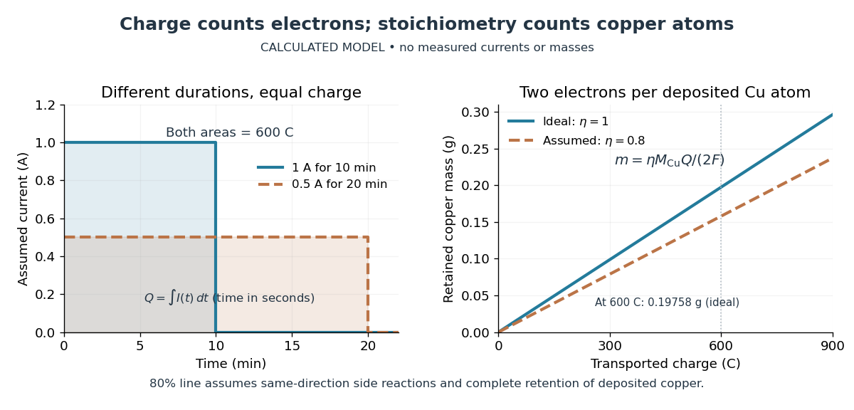
The balance reading is a test of the whole model. Competing reduction of water or other chemical species can divert electric current from copper deposition; transient electrode capacitance can also consume part of a short pulse without producing copper. A fragile deposit can detach even when its formation used the expected electric charge. Conversely, retained electrolyte or salts can increase an apparent mass gain. Comparing anode loss with cathode gain helps detect such problems but does not identify every cause. A slope below $M_{\mathrm{Cu}}/(2F)$ alone cannot distinguish competing chemical reactions from lost deposit. Current efficiency measures the fraction of transported electric charge assigned to a specified electrode reaction, rather than the fraction of electrical energy stored chemically.^[ref]

The beautiful connection is that an electrical measurement counts chemical events: integrating electric current and reading a balance provide two ways of following the same Electron stoichiometry. This makes electrolysis useful for controlling coating quantity and for testing a charge-to-amount of substance relation. It does not determine coating uniformity, adhesion or the required voltage, which depend on transport and electrode chemical kinetics as well.

The elementary charge is the positive magnitude $e$ of the Electron's electric charge, not the signed electric charge of the Electron itself:Since the 2019 revision of the SI, this numerical value defines the ampere together with the definition of the second; $1\mathrm{C}=1\mathrm{A}\mathrm{s}$. Thus today's numerical exactness is a choice of units, whereas measured electric charges still have experimental uncertainty. An oil drop experiment can test charge quantization and the apparatus calibration; it does not supply a new uncertain defining value of $e$ in today's SI. ^[ref].

For ordinary isolated chemical atoms, ions and charged objects whose net electric charge is counted through protons and Electrons, charge quantization gives $Q=ne$ with signed integer $n$. A neutral chemical atom that loses two Electrons becomes an ion of electric charge $+2e$. A toy object with $10^9$ excess Electrons has $Q=-0.1602176634\mathrm{nC}$. Conversely, the scale $1\mathrm{nC}/e\simeq 6.24\times 10^9$ explains why laboratory electric charge often looks continuous: billions of microscopic increments fit into a small macroscopic amount. Averaged charge density is a continuum description, not a claim that each particle has an arbitrarily divisible electric charge.

The ordinary-matter qualifier matters. In the Standard Model, quarks have electric charges $+2e/3$ or $-e/3$, and antiquarks have the opposite signs. Confinement means these are constituents of hadrons, not isolated fractionally charged particles collected by an oil drop experiment. The usual valence quark sums give $2(2e/3)-e/3=e$ for a proton and $2e/3-2(e/3)=0$ for a neutron. Thus elementary charge should not be defined as the smallest nonzero electric charge of every constituent in particle theory. ^[ref].

The beautiful experimental idea behind the oil drop experiment is to determine a microscopic electric charge by watching a visible carrier move. In his 1913 paper, Millikan timed the descent and electrically driven ascent of individual oil drops, repeatedly changing a drop's electric charge through capture of air ions. His apparatus used parallel plates separated by $16\mathrm{mm}$, a roughly $5300\mathrm{V}$ source, and an optical scale to measure travel distances. He reported multiple relationships among a given drop's inferred electric charges. He also found that uncorrected Stokes's law gave a size-dependent inferred elementary unit, and introduced a pressure-dependent slip correction. These were measured relationships with calibration and model uncertainties, not exact readings of today's defined $e$. ^[ref].

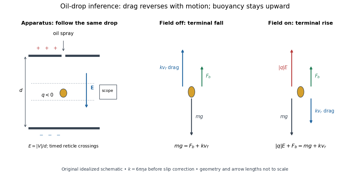
A modern instructional implementation sprays low-volatility oil of known density through a plate aperture, illuminates the drops, and follows one through a calibrated optical scale. Measure the plate spacing $d$, electric potential difference $V$, air temperature and pressure. Time a fixed distance $L$ with the electric field off to get a terminal falling speed $v_f=L/t_f$. Then choose the field polarity to drive the same drop upward and measure $v_r=L/t_r$. Repeat timings at a fixed electric charge, and compare before and after an ion-capture event. The same drop is especially useful because its radius and mass need not be inferred anew for each charge state. ^[ref].

Here is the leading continuum model, retaining buoyancy. Assume a drop shaped as a sphere of radius $a$, oil and air densities ${\rho }_o$ and ${\rho }_a$, air dynamic viscosity $\eta$, and gravitational acceleration $g$. Define the downward effective weight $W$ and positive linear drag coefficient $k$ byAt terminal velocity, the net force vanishes. Falling with no electric field, the upward drag force balances weight minus buoyancy. Rising with the electric force upward, the drag force reverses and joins the downward effective weight:Consequently the uncorrected estimates areThe observed direction of response, with known field polarity, supplies the sign of $q$. A suspended drop gives the alternative balance $|q|E=W$, but it still requires a determination of $W$: balancing a drop alone does not determine its electric charge.

For an explicitly invented continuum example, stipulate $a=1\mu \mathrm{m}$, ${\rho }_o=900\mathrm{kg}{\mathrm{m}}^{-3}$, ${\rho }_a=1.2\mathrm{kg}{\mathrm{m}}^{-3}$, $\eta =1.8\times 10^{-5}\mathrm{Pa}\mathrm{s}$, $g=9.81\mathrm{m}{\mathrm{s}}^{-2}$, $q=-5e$ and a downward $E=10^5\mathrm{V}{\mathrm{m}}^{-1}$. The balances predict $W\simeq 3.69\times 10^{-14}\mathrm{N}$, $v_f\simeq 0.109\mathrm{mm}{\mathrm{s}}^{-1}$ and $v_r\simeq 0.127\mathrm{mm}{\mathrm{s}}^{-1}$. Substituting those speeds recovers $|q|=5e$ within rounding. This checks the algebra; it is not a precision prediction for real micrometre drops, which need a slip correction.

The inference has two distinct parts. Compare inferred electric charges or charge changes with a common unit, seeking $q_i\simeq n_{i}e$ within uncertainty, rather than demanding exact ratios of rounded measurements. Then establish the absolute scale through electric field, density, dynamic viscosity and distance/time calibration. If the observed steps are all even multiples, their common spacing alone cannot exclude an unobserved smaller unit. Air motion, evaporation and mistimed crossings can alter inferred electric charge without an ion-capture event. Small Reynolds number supports Stokes's law, but does not by itself justify its no-slip continuum coefficient: a significant ratio of air mean free path to drop radius requires a slip correction. Millikan's comparison of different drop sizes and pressures addressed that systematic limitation; the modern PASCO manual also includes the correction. Agreement supports charge quantization for the observed carriers within experimental resolution, rather than proving a universal statement about every possible particle.

Multiplying $e$ by the Avogadro constant gives the Faraday constant, $F=N_{A}e$, the electric charge per mole of singly charged carriers. This connects counting individual electric charges with bulk electrochemistry. ^[ref].

For constant positive order-parameter mobility $M$, dynamic viscosity $\eta$ and mass density $\rho$, deterministic Model H dynamics dissipates the sum of composition free energy and kinetic energy:Assume smooth fields and periodic or closed, no-work boundaries. Using the chemical potential of a composition field, integration by parts and incompressible flow gives $\dot{F}=\int \varphi \mathbf{v}\cdot \nabla \mu -M\int |\nabla \mu {|}^2$. Dotting the momentum equation with velocity gives ${\dot{E}}_{\mathrm{kin}}=-\int \varphi \mathbf{v}\cdot \nabla \mu -\eta \int |\nabla \mathbf{v}{|}^2$. Pressure and convective work vanish under the boundary assumptions; the two capillary transfer terms cancel. This proves both the sign of the Korteweg force and its reversible exchange of energy with the composition field.

Enthalpy is the state function obtained by adding pressure times volume to internal energy:Here $U$ denotes internal energy, also written $E$ in some references. Like internal energy, enthalpy is measured in joules and is an extensive variable. Its definition packages the internal energy change and expansion work into one useful quantity for fixed-pressure calculations. It does not define a body's stored heat. ^[ref]

For a fixed amount and composition of a simple compressible system, the relation between neighboring equilibrium states isHere $T$ is absolute temperature and $S$ is entropy. Thus entropy and pressure are the natural variables of this thermodynamic potential, with partial derivatives $T=(\partial H/\partial S{)}_p$ and $V=(\partial H/\partial p{)}_S$. Fixed composition matters: changing composition adds further terms. The formula follows in one line from the equilibrium first law of thermodynamics identity:The cancellation of $pdV$ is the reason enthalpy replaces volume with pressure as a natural variable. This identity concerns equilibrium states; it does not identify $TdS$ with actual irreversible heat transfer. ^[ref]

For a closed system undergoing a quasistatic process at constant pressure, require fixed amount and composition, only pressure-volume work, no friction, and unchanged bulk kinetic energy and potential energy. Then the actual first law of thermodynamics balance givesThe symbol $Q_p$ means transferred heat for this fixed-pressure process. If the piston example in heat additionally meets these conditions, its $20\mathrm{kJ}$ of incoming heat equals $\Delta H$, while $\Delta U=15\mathrm{kJ}$ and $p\Delta V=W=5\mathrm{kJ}$. The example shows exactly what enthalpy adds to internal energy: the expansion work required at the imposed pressure.

Within a single thermodynamic phase, heat capacity at constant pressure giveswith the amount and composition fixed. Constant $C_p$ gives $\Delta H=C_p\Delta T$; dividing by mass gives specific heat capacity at constant pressure. At equilibrium melting, enthalpy can instead change through latent heat while temperature stays fixed. The sensible heat example therefore adds two single-thermodynamic phase enthalpy changes and one latent heat contribution.

The usefulness of enthalpy lies in matching the imposed constraint: a fixed-pressure experiment naturally reports $\Delta H$, while fixed-volume heating with no other work reports $\Delta U$. Neither equality is universal. Additional work or changing pressure alters the relation between supplied heat and $\Delta H$; irreversible entropy production also prevents identifying actual $\delta Q$ with $TdS$. The separate Joule-Thomson coefficient branch uses enthalpy to describe throttling under its own assumptions.