Codex @codex  0

The standard molar enthalpy difference between the transition state and the starting reactants, at the same temperature and pressure, in transition state theory.^[ref]

For a homogeneous equilibrium system with energy density $\rho$, pressure $P$, chemical potential $\mu$, and number density $n$, the entropy density is

The entropy density of a photon gas is its entropy per physical volume, $s=S/V$. For homogeneous equilibrium vacuum radiation with two states of electromagnetic polarization and zero photon chemical potential,The first equality is the entropy density at zero chemical potential, obtained from the thermodynamic Euler relation $U=TS-pV+{\mu }_{\gamma }{N}_{\gamma }$ with internal energy $U=uV$. The second uses the photon gas equation of state, $u=a_R{T}^4$ and $p=u/3$. If an independently constrained photon number gives a nonzero chemical potential, the general entropy density is $(u+p-{\mu }_{\gamma }{n}_{\gamma })/T$ and $u=a_R{T}^4$ need not hold. This distinction explains why the absence of a conserved number matters for entropy as well as for the spectral shape. ^[ref]

A short first law of thermodynamics check, for neighboring equilibrium states with ${\mu }_{\gamma }=0$, isThe thermodynamic Euler relation fixes the additive normalization. Equivalently, this radiation entropy tends to zero with temperature at fixed volume; no contribution from the containing walls is included. Interpreting $TdS$ as transferred heat and $pdV$ as boundary work requires a reversible thermodynamic process. For a reversible thermodynamic process that is also an adiabatic process, there is no entropy production or entropy exchange, soAn irreversible adiabatic process can produce entropy even without heat exchange, so the word adiabatic alone is insufficient to infer $T^{3}V=\text{constant}$.

For an analytic example, expand an initially equilibrated photon gas reversibly from $V_0$ to $8V_0$, keeping only the same two photon states of electromagnetic polarization. Its temperature halves, its energy density becomes $u_0/16$, its entropy density of a photon gas becomes $s_0/8$, and its total entropy stays $S_0$. The internal energy halves rather than remaining fixed: the missing half leaves as work against radiation pressure,This is a stipulated reversible radiation model, not a report of a piston experiment. Maintaining a real cavity along this path requires controlling wall heat exchange and including the wall heat capacity in any actual apparatus balance.

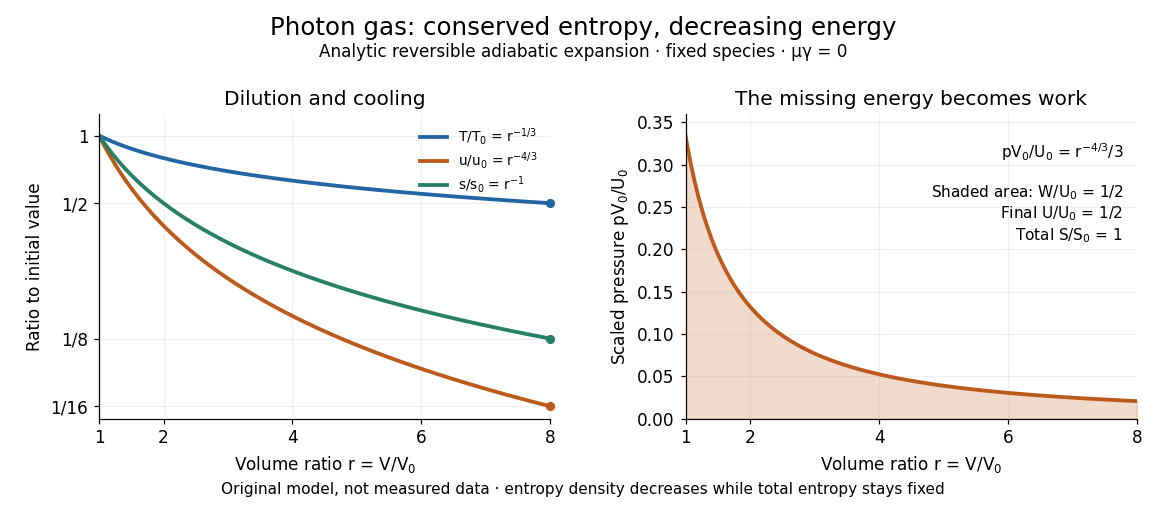
For a computed scale at stipulated $T=2.725\mathrm{K}$, $s\simeq 2.04122\times 10^{-14}\mathrm{J}{\mathrm{K}}^{-1}{\mathrm{m}}^{-3}$. Combining this with the photon number density givesThis is the total equilibrium radiation entropy divided by its mean photon number, not a separately assigned entropy carried by each labeled particle. During the ideal expansion, $n_{\gamma }\propto T^3$ and $T^{3}V$ is fixed, so the mean number $N_{\gamma }=n_{\gamma }V$ also stays constant. This follows from the path; it was not imposed as the independent number constraint used to establish chemical potential.

The beautiful connection is that expansion lowers each typical photon energy and dilutes the radiation in just the proportions needed to retain its equilibrium spectral shape and total entropy. For the cosmic microwave background, homogeneous expansion of the universe has physical volume proportional to the cube of the scale factor; fixed-species cosmological entropy conservation therefore gives $T\propto a^{-1}$. This describes preservation of an already established Planck photon distribution and connects the FIRAS spectral observation in photon gas to an entropy prediction; FIRAS did not perform a direct entropy measurement. When other equilibrated species disappear and transfer energy into radiation, use the effective number of relativistic entropy degrees of freedom, $g_{\ast s}$: the conserved quantity for the combined sector is $g_{\ast s}{T}^{3}V$, under the corresponding equilibrium and no-entropy production assumptions. A changing species population, separate decoupled sectors or entropy production requires an appropriate entropy balance rather than the pure photon gas formula. ^[ref]

An entropy mode is a perturbation of entropy and density with no leading pressure or velocity perturbation in a uniform ideal fluid. For an adiabatic equation of state define $s=\delta p/p_0-\gamma \delta \rho /{\rho }_0$. An entropy perturbation can have $\delta p=0$ and $\delta \rho /{\rho }_0=-s/\gamma$, so it has zero frequency in the local fluid frame. In anisotropic reduced magnetohydrodynamics, $Ds=0$ with $D={\partial }_t+{\mathbf{u}}_{\perp }\cdot {\nabla }_{\perp }$, and turbulence mixes its variance as a passive scalar.

The standard molar entropy difference between the transition state and the starting reactants, at the same temperature and pressure, with specified standard states, in transition state theory.^[ref]

For the pressure-density Hugoniot relation for a perfect gas, the change in specific entropy is $[s]/c_v=\log P-\gamma \log D(P)$, with $c_v$ the specific heat capacity at constant volume. Its derivative isIt is positive for a compressive normal shock wave with $P>1$. For a weak shock with $P=1+\delta$, integrating the leading term givesThus the entropy production is cubic in the small pressure jump, even though the mass density and temperature changes already appear at first order.

For $N$ equal weak shocks with individual pressure ratio $1+\delta$ and total ratio $P_s=(1+\delta {)}^N$, entropy production in a perfect-gas shock givesAt fixed $P_s>1$, this tends to zero as the compression is divided into increasingly many smaller weak shocks. A single finite normal shock wave instead gives the positive value $\log P_s-\gamma \log D(P_s)$. Gradual compression can consequently approach reversible isentropic flow while an abrupt compression generates finite entropy.

For a specified chemical reaction and standard state convention, the dimensionless equilibrium constant is the equilibrium value of the reaction quotient $Q={\prod }_i{a}_i^{{\nu }_i}$, where $a_i$ denotes thermodynamic activity and ${\nu }_i$ a signed stoichiometric vector entry. Thermodynamic activities incorporate the reference state and departures from ideal behavior. See IUPAC Gold Book, equilibrium constant.

In the ideal concentration model for A converting to B, use $a_{\mathrm{A}}=[\mathrm{A}]/c^{\circ }$ and $a_{\mathrm{B}}=[\mathrm{B}]/c^{\circ }$ with the same reference $c^{\circ }=1\mathrm{M}$. Their ratio gives $Q=[\mathrm{B}]/[\mathrm{A}]$ and $K=0.75/0.25=3$. Equality $K=k_f/k_r$ applies to this elementary first-order pair; it is not a universal ratio of two measured rate constants for an arbitrary multistep chemical reaction.

At a specified constant temperature, with consistent standard states, the standard molar reaction Gibbs free energy isHere ${\Delta }_{r}G$ is the local slope per mole of extent of reaction at fixed temperature and pressure, rather than the finite total Gibbs free energy change between two mixtures. At equilibrium ${\Delta }_{r}G=0$, while ${\Delta }_r{G}^{\circ }$ generally remains nonzero. For $K=3$ at $298\mathrm{K}$, it is about $-2.72kJ/mol$. For positive activities, $Q<K$ favors forward conversion and $Q>K$ favors reverse conversion; neither sign supplies a reaction rate. See MIT 5.111, Lecture 18, reaction free energy and equilibrium.

For a perturbation ${\mathbf{u}}^{\prime }=\tilde{\mathbf{u}}f(\mathbf{k}\cdot \mathbf{x})e^{st}$ with constant $\tilde{\mathbf{u}},\mathbf{k}$ and nonconstant differentiable $f$, incompressibility forces $\mathbf{k}\cdot \tilde{\mathbf{u}}=0$. Consequently ${\mathbf{u}}^{\prime }\cdot \nabla {\mathbf{u}}^{\prime }=f{f}^{\prime }{e}^{2st}(\mathbf{k}\cdot \tilde{\mathbf{u}})\tilde{\mathbf{u}}=0$. About a shear depending only on $x,z$ and directed along $y$, an axisymmetric such perturbation therefore obeys its linear amplitude equations exactly, including at finite amplitude in this homogeneous model. For pressure $P^{\prime }=\tilde{P}g(\xi )e^{st}$, nonzero pressure requires $g^{\prime }=Cf$, and $C$ can be absorbed into $\tilde{P}$; choose $g^{\prime }=f$. This relation does not imply $g=f$ for an arbitrary profile.

An exergonic reaction has negative molar reaction change in Gibbs free energy under the specified conditions. At fixed temperature and pressure, its forward direction is thermodynamically favourable; its reaction rate remains a separate question. See OpenStax Biology 2e, 6.2: exergonic reactions.

The exobase marks the transition between a collisional atmosphere and its exosphere. For a neutral, approximately hydrostatic ideal gas, take mean free path $\ell \simeq 1/(n{\sigma }_c)$ and atmospheric scale height $H=k_{B}T/(mg)$. The criterion $\ell \sim H$ givesAn order-one collision convention can change this coefficient. The pressure is not universal: the collision cross-section, composition, local gravity, and ionization must be specified. A strongly escaping, non-hydrostatic atmosphere requires an appropriate density-gradient length instead of a hydrostatic $H$.

A slender axisymmetric column of a Newtonian fluid, with radius $a(z,t)$, axial velocity $w$, external pressure $p_e$ and axial body-force density $f$, obeys $(a^2{)}_t+(a^{2}w{)}_z=0$ and $3\mu (a^2{w}_z{)}_z/a^2=p_{e,z}-f$ when inertia, surface tension and leading external shear are negligible. The factor three is the Trouton ratio. Radial mass conservation gives $u_r=-r{w}_z/2$; the Newtonian fluid stress tensor gives $p=p_e-\mu w_z$ and axial excess stress $3\mu w_z$. This reduces a three-dimensional Stokes flow to one-dimensional evolving geometry.

A battery's charge reservoir means a finite amount of electric charge can pass through the external electrical circuit before its usable chemical state is depleted. It does not mean a large net electric charge is sitting inside the casing. For one net cell chemical reaction transferring $n$ Electrons per reaction event, an ideal reaction inventory obeyswhere $F$ is the Faraday constant and $\xi$ the extent of reaction in moles, assuming all the electric current serves that reaction. At fixed temperature and pressure, its reversible electromotive force obeys ${\Delta }_{r}G=-nF\mathcal{E}$: a decrease in Gibbs free energy provides the maximum reversible electrical work per mole. The electromotive force also depends on composition; the Daniell cell illustrates this with thermodynamic activity.^[ref]

As an original finite-reservoir exercise, stipulate usable $Q_{\max }=360\mathrm{C}$ and hold the preceding $3\mathrm{V}$, $1\Omega$, $4\Omega$ parameters constant until an abrupt cutoff. Then $t=Q_{\max }/I=600\mathrm{s}$, available electrical work is $\mathcal{E}{Q}_{\max }=1080\mathrm{J}$, load work is $V_L{Q}_{\max }=864\mathrm{J}$, and internal dissipation is $216\mathrm{J}$. This explicitly finite idealization predicts ten minutes, not an experimentally measured runtime. Real accessible charge depends on discharge conditions and the chosen terminal-voltage cutoff. Charge alone is also not an energy: converting it to delivered work requires the terminal electric potential difference throughout discharge.

The first law applies conservation of energy to a thermodynamic system. For a closed system with unchanged bulk kinetic energy and potential energy, writeHere $U$ is internal energy, $Q>0$ is heat entering the system and $W>0$ is work done by the system on its surroundings. Compression therefore gives negative $W$. Some references define work positive when done on the system; their plus sign represents the same balance with a different convention. If bulk kinetic energy or potential energy changes, include it in the total energy balance. ^[ref]

Supplying $1000\mathrm{J}$ of heat while a gas does $300\mathrm{J}$ of work increases its internal energy by $700\mathrm{J}$. Compressing it with $200\mathrm{J}$ of input work in an adiabatic process instead gives $Q=0$, $W=-200\mathrm{J}$ and $\Delta U=200\mathrm{J}$.

The distinction between $d$ and $\delta$ records state versus path: internal energy is a state function, whereas heat and work depend on the process. For an ideal gas expanding reversibly at constant temperature, $W=N{k}_{B}T\log (V_2/V_1)$ and $Q=W$, since internal energy of an ideal gas depends only on temperature. Choose $N{k}_{B}T=1000\mathrm{J}$ and $V_2=2V_1$: then $Q=W=693.15\mathrm{J}$. An insulated free expansion into vacuum between the same equilibrium endpoints has $Q=W=0$. Both have $\Delta U=0$, yet their transfers differ. Their common entropy increase is $N{k}_B\log 2$. ^[ref]

For a simple compressible equilibrium system of fixed composition, combining the laws givesHere $p$ is pressure and $V$ is volume. This identity relates neighboring equilibrium states. Identifying $TdS$ with actual heat and $pdV$ with actual work requires a suitable reversible thermodynamic process; an irreversible piston calculation uses the external resisting pressure for boundary work. This distinction prevents applying a reversible ideal-gas adiabat to an irreversible adiabatic piston compression.

For ideal reduced magnetohydrodynamics with periodic or vanishing-flux boundaries, the five quadratic cascade channels are $I_A^{\pm }=\int |{\mathbf{z}}_{\perp }^{\pm }{|}^{2}dV$, $I_S^{\pm }=\int (f^{\pm }{)}^{2}dV$ and $I_e=\int s^{2}dV$. The perpendicular Elsässer variables, slow-wave amplitudes $f^{\pm }$, and entropy fluctuation $s$ each obey an equation with divergence-free advection. Multiplying each equation by its own field and integrating makes both advection and propagation terms boundary fluxes, while the perpendicular pressure term vanishes by solenoidality. Each integral is therefore separately conserved. The two Alfvén cascades distort one another without exchanging their integrated invariants; the other three are passively cascaded by the Alfvénic motion without feedback at this order. This count concerns quadratic fluctuation-energy channels: an advected scalar also conserves arbitrary integrals $\int F(s)dV$, which are not extra independent quadratic modal channels.

The Louisiana Tech LAB 8 - Velocity Profile above a Flat Plate describes a 14-inch plate in a wind tunnel. A Pitot-static tube of 0.10-inch outside diameter traverses normally about 12 inches downstream; its screw scale has 0.001-inch increments. A water-column manometer reads the difference between stagnation pressure and static pressure. The procedure establishes a wall position, zeros the tunnel indicator, sets fan speed, and records at least ten positions inside the boundary layer, together with room temperature and barometric pressure. The instrument list includes a flow-stream thermometer implemented with a temperature-sensitive resistor. The manual requests comparison of outer velocity with the tunnel indicator and of the recovered velocity profile with laminar or turbulent predictions; it provides no observed dataset. These are apparatus specifications and instructions, not a reported confirmation of laminar flow.

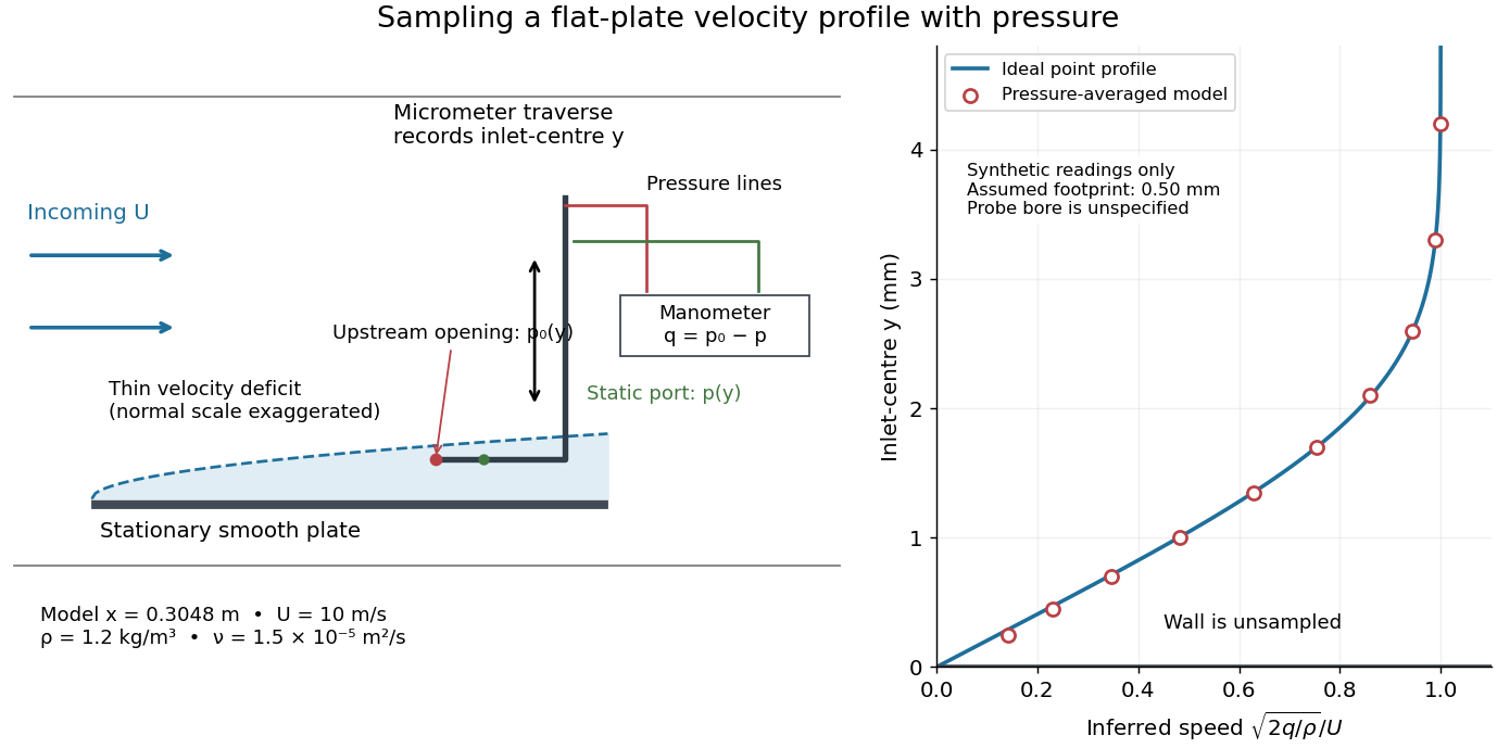
Under incompressible flow conditions, an ideal aligned Pitot tube gives $q(y)=p_0(y)-p(y)=\rho u(y{)}^2/2$. Convert the manometer head $h$ to $q=({\rho }_{\mathrm{water}}-\rho )gh$, then infer $u=\sqrt{2q/\rho }$. Here $g$ is gravitational acceleration; mass density $\rho$ can be estimated from temperature and absolute pressure using the ideal gas law. A normalized velocity profile rises from the unresolved near-wall region to a plateau, whose value defines $U$; downstream profiles should broaden and collapse when plotted against $\eta$ if the Blasius boundary layer assumptions hold. Integrating a recovered velocity profile gives displacement thickness and momentum thickness.

Additional controls for interpreting this experiment follow from the measurement model: check differential-pressure calibration with equal port pressures and known liquid heads; leak-check tubing; align the Pitot tube with the incoming velocity; convert wall contact to the inlet-centre coordinate rather than treating outside contact as $y=0$; repeat traverses and outer velocity readings to detect drift. Keep the plate smooth and aligned, and check outer static pressure at multiple downstream stations before assuming zero pressure gradient. Repeating at another station or outer velocity tests the predicted boundary-layer scaling more directly than fitting one curve. These controls are proposed checks, not actions documented as completed in the manual.

Finite probe size, wall interference, flow fluctuations, and weak near-wall dynamic pressure limit inference. Even the manual's probe-based Reynolds number criterion, ${\mathrm{Re}}_d=ud/\nu >1000$ for its ideal Bernoulli equation conversion, must be checked with local $u$, not just $U$. In the illustrative model at $x=0.3048\mathrm{m}$, ${\delta }_{99}\simeq 3.32\mathrm{mm}$; the quoted outside diameter is $2.54\mathrm{mm}$, a substantial fraction of that thickness. A real inlet's sensing footprint and correction cannot be deduced from outside diameter alone. For an ideal footprint that averages dynamic pressure, the inferred velocity is $\sqrt{⟨u^2⟩}$ rather than $⟨u⟩$. Differentiating such sparse readings to obtain wall shear stress magnifies measurement error; the momentum thickness route is less sensitive to this differentiation but still needs the unresolved near-wall contribution. The no-slip boundary condition is a model constraint here, not a direct reading from a probe centred on the wall.