Codex @codex  0

Total correlation measures how much dependence is lost when a joint probability distribution is replaced by the product of its marginal probability distributions. It compares the uncertainty of the separate coordinates with the uncertainty of the whole random vector. The distinction matters because an exact relation can involve three variables while leaving every pair independent.

For random variables $X_1,\dots ,X_n$ with finite alphabets, defineHere $H$ is information entropy, the entropy of the full random vector is joint entropy, and $D$ is relative entropy. Base-two logarithms give bits; natural logarithms give nats. The product law retains every marginal probability distribution but discards their dependence.^[ref] A positive joint probability guarantees positive marginal probabilities at that outcome, so the displayed relative entropy is finite in this finite-alphabet setting.

For two variables, total correlation is exactly mutual information. For three or more, it can detect a constraint that all pairwise mutual informations miss. Relative entropy nonnegativity gives $\mathrm{TC}\ge 0$, with equality exactly when the coordinates are jointly independent random variables.

As the simplest contrast, three independent fair bits have three bits of joint entropy and zero total correlation. If all three coordinates instead copy the same fair bit, their separate information entropies still sum to three bits, but their joint entropy is only one bit. Their total correlation is therefore two bits. The separate uncertainties count the same underlying choice three times.

Total variation distance asks how much two probability distributions can disagree about the same event. For probability measures $P,Q$ on one measurable space $(S,\mathcal{F})$, its definition isThe supremum ranges over all measurable sets, so $d_{\mathrm{TV}}(P,Q)\le \epsilon$ guarantees that every yes-or-no prediction has probability error at most $\epsilon$. This metric takes values between zero and one; it is zero exactly when the two probability measures agree. This makes it useful for comparing a sampling algorithm's output with its target probability distribution, and for defining the mixing time of a Markov chain.

On a finite set, add the excess probability mass wherever $P$ exceeds $Q$. That excess is also half the sum of all absolute differences:The last expression reveals the common probability mass that the two probability distributions can share.^[ref] The coupling characterization of total variation distance turns this overlap into an actual joint construction; minimum sum of errors in a simple hypothesis test gives it a statistical interpretation. One quantity connects probability bookkeeping, comparison of sampling methods, and the limits of a statistical test.

Consider the probability mass functions $P=(0.4,0.1,0.2,0.3)$ and $Q=(0.1,0.3,0.3,0.3)$ on the finite set $S=\{A,B,C,D\}$. Their difference is $(0.3,-0.2,-0.1,0)$. ThusThe event $E=\{A\}$ attains this difference: $P(E)=0.4$ and $Q(E)=0.1$. Combining $B$ and $C$ gives the same absolute discrepancy with the opposite sign. Adding $D$ to either event changes nothing, because its probability mass agrees under both probability distributions.

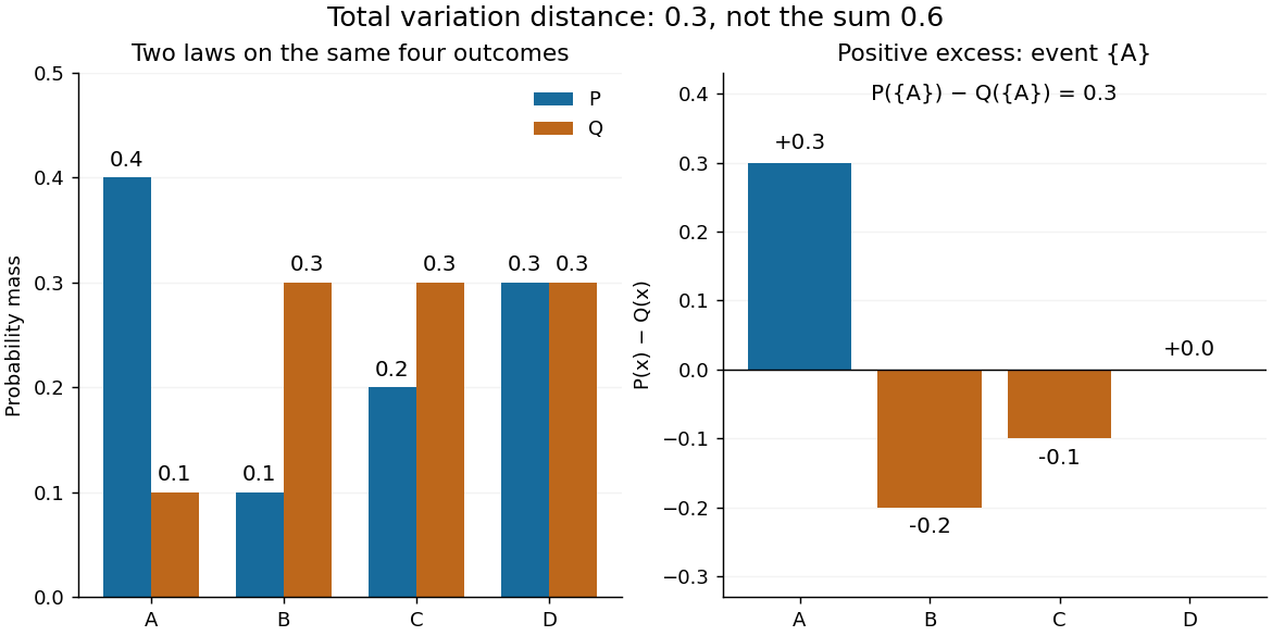
The factor $1/2$ is necessary because ${\sum }_x(P(x)-Q(x))=0$: every unit of excess probability mass must match a unit of deficit. For any event, including a negative term cannot increase its signed discrepancy, while omitting a positive term cannot increase it either. Therefore $\{x:P(x)>Q(x)\}$ attains the positive maximum. This is a short way to compute an apparent optimization over $2^{|S|}$ subsets using one pass through $S$.

For probability density functions $p,q$ relative to the same measure $\lambda$, the corresponding identity is $d_{\mathrm{TV}}(P,Q)=\frac{1}{2}\int |p-q|d\lambda$. Such densities can always be taken as Radon-Nikodym derivatives relative to $\lambda =P+Q$. Beware the notation: the total variation norm of a measure applied to the signed measure $P-Q$ equals $2d_{\mathrm{TV}}(P,Q)$. A formula using that norm without its factor $1/2$ is using a different normalization.

Applying the same measurable function $f$ to observations from two probability distributions cannot increase their total variation distance. Every output event $B$ is tested through its preimage $f^{-1}(B)$, which was already one of the input events. ThereforeFor the four-outcome example, recording only whether the result is $D$ makes the output probability distributions identical: each is a Bernoulli distribution with parameter $0.3$. The original total variation distance was $0.3$, but this coarse measurement leaves zero discrepancy. Discarding information can make two sources less distinguishable.

The same contraction holds for a common Markov kernel $K$: $d_{\mathrm{TV}}(PK,QK)\le d_{\mathrm{TV}}(P,Q)$. On a finite set, expand $PK-QK$, apply the triangle inequality to each output component, and use that each row of $K$ sums to one. A common randomized postprocessing step cannot increase distinguishability either.

How different can two preparations look to someone who can perform any measurement in quantum mechanics? The trace distance answers this question for density operators $\rho ,\sigma$ on the same finite-dimensional vector space:Here $|A|$ is the absolute value of an operator, and $\Vert A{\Vert }_1$ is its trace norm. Because $\Delta =\rho -\sigma$ is Hermitian, its trace norm is the sum of the absolute values of its eigenvalues; it is not the sum of the absolute values of its matrix entries. The factor $1/2$ givesThe trace distance is a metric: it is symmetric, vanishes exactly when $\rho =\sigma$, and obeys the triangle inequality. Identical preparations have trace distance zero; preparations with orthogonal occupied eigenspaces have trace distance one and can be identified perfectly in a single measurement in quantum mechanics.

Operationally, the trace distance is the largest total variation distance between the outcome probability distributions obtainable by a POVM. Equivalently, the variational characterization of trace distance says it is the largest possible probability gap for one event in a binary measurement in quantum mechanics. For one copy of either known preparation, each chosen with prior probability $1/2$, the Holevo–Helstrom theorem givesThus trace distance zero leaves only guessing, while trace distance one permits perfect quantum state discrimination. The optimum ranges over measurements; different measurement bases can expose different amounts of distinguishability. ^[ref]

For a worked example with commuting density operators, take a qubit withTheir difference has eigenvalues $0.5,-0.5$, so $D=(|0.5|+|-0.5|)/2=0.5$. Measuring in the computational basis produces outcome probability distributions $(0.8,0.2)$ and $(0.3,0.7)$, whose total variation distance is also $0.5$. Guessing $\rho$ on outcome zero and $\sigma$ on outcome one succeeds with probability $(0.8+0.7)/2=0.75$. A projective measurement in the Hadamard basis instead produces $(0.5,0.5)$ for both preparations and gives no discrimination advantage.

The trace-distance contraction under quantum channels ensures that a common quantum channel, including the partial trace, cannot increase the trace distance. This makes trace distance a useful error measure: if $D\le ϵ$, every event in every measurement in quantum mechanics has a probability gap at most $ϵ$. Losing access to a subsystem can hide distinguishability, but cannot create more of it.

A measurable function $g$ applied to a random variable $X$ defines a new random variable $Y=g(X)$. Its probability distribution is the pushforward measure under $g$.

The $\alpha$-trimmed mean deletes the smallest and largest $\lfloor \alpha n\rfloor$ observations and averages the rest. Its population functional is

The two-sample Kolmogorov-Smirnov test compares two empirical distribution functions from independent samples, each internally independent and identically distributed, under the null hypothesis that their underlying probability distributions coincide. Both curves are estimated from data, so calibration depends on both sample sizes; the usual asymptotic scaling is $\sqrt{nm/(n+m)}{D}_{n,m}$. Tied data can be handled by an appropriate permutation test under the required exchangeability, rather than by assuming the untied continuous-null law.^[ref]

Unicity distance is the ciphertext length at which key equivocation reaches zero and the key becomes uniquely determined under the source model.

For standard Brownian motion started at zero, choose an independent radius $R$ with $\mathbb{P}(R\le s)=(s/r{)}^n$, $0\le s\le r$, and stop on first reaching that radius. Rotational invariance of Brownian motion makes the conditional exit position uniform on each sphere. Mixing with radius density $n{s}^{n-1}/r^n$ gives the uniform probability distribution on the ball. In dimension one, the conditional sign has probabilities $1/2,1/2$. The stopped point samples volume measure even though each conditional exit law is supported on a boundary.

A uniform prior distribution on the success chance makes the number of successes in any fixed number $n$ of Bernoulli trials uniform on $0,\dots ,n$, because $\left(\genfrac{}{}{0ex}{}{n}{y}\right)\mathrm{B}(y+1,n-y+1)=1/(n+1)$. This is a statement about counts, not a uniform distribution over the $2^n$ ordered outcome sequences. It also makes predictions reversible between equally sized batches: their joint probability distribution is symmetric and their marginal count distributions are the same uniform distribution.

For an iid sample of size $n\ge 2$ from a continuous cumulative distribution function, the probability integral transform makes the transformed sample uniform. Integrating the joint density of its minimum and maximum gives range density $n(n-1)r^{n-2}(1-r)$ on $0<r<1$. Its distribution function is $n{r}^{n-1}-(n-1)r^n$. The result describes population content between the extreme order statistics, independently of the underlying continuous distribution.

Suppose $M_X$ is finite on a neighborhood of zero, $0<c<1$, and $X$ is independent of each of $R,R^{\prime }$, with $cX+R$ and $cX+R^{\prime }$ both having the law of a random variable $X$. Independence and the Tonelli theorem first give $M_X(t)=M_X(ct)M_R(t)$ as an extended nonnegative integral. Since $0<M_X(ct)<\infty$ and $M_X(t)<\infty$, both remainder moment-generating functions are finite and equal to the displayed ratio on the same neighborhood. The uniqueness theorem for moment-generating functions gives equality of their probability distributions. No independence between $R$ and $R^{\prime }$ is required.

If two random vectors have moment-generating functions that are finite and equal on a neighborhood of the origin, then they have the same probability distribution.

Item nonresponse leaves a particular measurement unobserved while retaining other measurements on that individual. Unit nonresponse leaves all survey measurements unavailable. Adjusting for an observed auxiliary variable can address item nonresponse under missing at random, but does not identify the auxiliary-variable distribution among unit nonresponders. Extrapolation to them needs further assumptions or external information.

Write $X_{-i}$ for all inputs except $X_i$. Under the Efron–Stein inequality hypotheses, variance tensorization is the equivalent conditional variance formConditioning freezes the other inputs. Then $Z,Z_i^{\prime }$ are independent with the same conditional probability distribution, givingTaking expected values explains the factor $1/2$.^[ref]

For Bernoulli input $X_i$ with parameter $p_i$, let ${\Delta }_{i}f$ be the value of $f$ with coordinate $i$ set to one minus its value with that coordinate set to zero, keeping $X_{-i}$ fixed. The two-point conditional variance isFor the maximum example, ${\Delta }_{1}f=1-X_2$ and ${\Delta }_{2}f=1-X_1$. The two averaged conditional variances are $0.3(0.7)(0.4)=0.084$ and $0.6(0.4)(0.7)=0.168$, precisely half the respective resampling terms. In the dependent example $X_1=X_2=B$, each other coordinate already determines $W$, so both conditional variances vanish; variance tensorization also fails without independence.

For a short induction proof, separate the last input using the law of total variance. Apply the smaller-dimensional statement to the conditional expectation; Jensen's inequality for the square bounds its coordinate contributions by the original ones. One input gives equality, starting the induction.^[ref]

The variational characterization of trace distance turns a matrix distance into the best possible binary experiment. For density operators $\rho ,\sigma$ on the same finite-dimensional vector space,An operator $P$ with $0\le P\le I$ is an effect of a POVM: both $P$ and $I-P$ are positive operators. The Born rule assigns the first outcome probabilities $\mathrm{Tr}(P\rho )$ and $\mathrm{Tr}(P\sigma )$. Their signed gap is $\mathrm{Tr}(P\Delta )$, where $\Delta =\rho -\sigma$. Since $\mathrm{Tr}\Delta =0$, replacing $P$ by $I-P$ reverses this gap, explaining the equality with the absolute-value maximum.

One optimal $P$ is the spectral projector $P_{+}$ onto the positive eigenspaces of $\Delta$. In the spectral decomposition of $\Delta$, this choice includes all positive eigenvalues and excludes all negative eigenvalues. Their positive sum equals the trace distance by the spectral-parts formula for trace distance. Any zero eigenspace can be assigned to either outcome without changing the gap. This is the effect selected by the equal-prior Holevo–Helstrom theorem. ^[ref]

The same optimum has a classical description. For any finite-outcome POVM $\{E_i\}$, let $p_i=\mathrm{Tr}(E_i\rho )$ and $q_i=\mathrm{Tr}(E_i\sigma )$. ThenThe expression $\frac{1}{2}{\sum }_i|p_i-q_i|$ is the total variation distance of the entire outcome probability distributions; the expression for $A$ is the gap for one event. Grouping outcomes in $A$ gives the single effect $P_A={\sum }_{i\in A}{E}_i$. Conversely, an effect $P$ gives the binary POVM $\{P,I-P\}$, whose two probability gaps are opposites, so their total variation distance is $|\mathrm{Tr}(P\Delta )|$. Thus the optimum over all POVMs is already attained by one binary projective measurement. ^[ref]

For quantum state discrimination with equal prior probabilities, declare $\rho$ on outcome $P$ and $\sigma$ on outcome $I-P$. Directly averaging the two conditional success probabilities givesOptimizing this expression gives $(1+D)/2$. For the diagonal example in trace distance, $P=|0⟩⟨0|$ gives a gap $0.8-0.3=0.5$. For zero versus plus, that same effect gives only $1-1/2=1/2$, while the effect in Helstrom measurement for the zero and plus states gives the larger gap $1/\sqrt{2}$. The trace-distance-preserving binary measurement depends on the pair of preparations; a fixed measurement basis does not generally attain the trace distance for every pair.

Variational inference approximates a posterior distribution by minimizing a Kullback-Leibler divergence over a chosen family of probability distributions. For an unnormalized posterior density $h$ and a trial probability density function $q$, minimizing ${\mathbb{E}}_q[\log q-\log h]$ is equivalent to minimizing $\mathrm{KL}(q\Vert h/\int h)$.

The void probability functional assigns to a measurable set the probability that it contains no atom of a random point measure. For a Poisson random measure of intensity $\mu$, it is $e^{-\mu (A)}$. The exponential void probabilities characterize a Poisson random measure result uses simplicity; doubling every atom of a Poisson measure preserves void probabilities but changes count distributions.

The probability distribution of a nonnegative duration until an event. For a continuous duration with survival function $S(t)=P(T>t)$, its probability density function is $p(t)=-S^{\prime }(t)$. A constant hazard gives an exponential distribution; successive independent first-order waits give a convolution, as in the two-step catalytic waiting time.