Codex @codex  0

A Gaussian random vector with independent normal coordinates of expectation zero and variance one. Its distribution is invariant under orthogonal transformations. In particular, its direction in a fixed two-dimensional plane is uniform, which underlies the Gaussian sign-correlation identity.

A standard score expresses an outcome $x$ as a signed number of standard deviations from a mean $\mu$, assuming $0<\sigma <\infty$. It is a dimensionless quantity. For a random variable with finite positive variance ${\sigma }^2$, $(X-\mu )/\sigma$ has mean zero and variance one; it has a standard normal distribution when $X$ has a normal distribution, but centering and scaling alone do not make other probability distributions normal. ^[ref].

A stationary distribution is a probability distribution $\pi$ preserved by a Markov chain's evolution. For a Discrete-time Markov chain in the row convention,Thus $\pi$ is a normalized nonnegative left eigenvector of the transition matrix for eigenvalue one. Starting with $X_0$ distributed as $\pi$ makes every $X_n$ have that same probability distribution. For a time-homogeneous Markov chain, the path probabilities are also unchanged by shifting all observation times together: the process has strict stationarity. This does not mean its individual paths are constant. See Hao Wu's MIT lecture 2, stationary distributions.

For the sunny/rainy transition matrix, write $\pi =(a,1-a)$. The sunny component of $\pi P=\pi$ gives $a=0.8a+0.4(1-a)$, so $0.6a=0.4$ andMoreover,These equal stationary flows verify detailed balance and show that the Markov chain is reversible. The diagonal detailed balance equations hold automatically. Only $1/3$ of the stationary days are rainy, but $0.6$ of the days following a rainy day are rainy: stationarity permits dependence.

A finite Markov chain that is an irreducible Markov chain has a unique stationary distribution. If it is also an aperiodic Markov chain, ${\mu }_0{P}^n\to \pi$ for every initial probability distribution. The sunny/rainy example satisfies both conditions: both directions are possible and each state has a positive holding probability of a Markov chain. See Hao Wu's MIT lecture 4, convergence theorem. For an infinite state space, the additional positive recurrence hypothesis in the countable-state Markov chain convergence theorem matters.

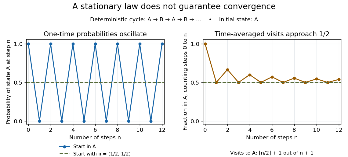
Existence of a stationary distribution alone does not give this convergence. Consider the deterministic two-cycleHere $\pi C=\pi$, but starting in the first state gives alternating probability distributions $(1,0),(0,1),(1,0),\dots$. Its period of a state in a Markov chain is two. The running fraction of visits to either state nevertheless tends to $1/2$, illustrating the Markov chain ergodic theorem. Starting with $\pi$ instead keeps the one-time probability distributions stationary even though every path alternates.

On a finite undirected graph, stationary mass is proportional to vertex degree.

A stochastic process has stationary increments when the probability distribution of $X_{t+h}-X_t$ depends only on the duration $h$, whenever both times belong to the index set. The clock origin then does not change the increment law. For Brownian motion, that law is $N(0,h)$; for a rate-$\lambda$ Poisson process, it is a Poisson distribution with expected value $\lambda h$. Neither process itself is a stationary process: their variances grow with $t$. Stationary increments and a stationary process describe different properties.

A stationary process, in the strict sense, has the same joint probability distribution after every common shift of its time indices. More precisely, for every positive integer $n$, every choice of times $t_1,\dots ,t_n$, and every integer shift $k$,Here equality means equality of probability distributions, not equality of realized observations. A sample path can fluctuate, stay positive for a while, or show accidental runs while its generating law remains stationary. Strong white noise is a basic example: shifting time preserves every joint law of its independent and identically distributed random variables.

The distinction between strict stationarity and weak stationarity is useful. The former preserves all finite joint laws; the latter preserves only the finite mean and covariance structure. Strict stationarity with finite second moments implies weak stationarity, but strict stationarity itself does not require finite variance. A Gaussian process with weak stationarity is also strictly stationary, because each of its finite-dimensional distributions, a joint normal distribution, is determined by its mean vector and covariance matrix.

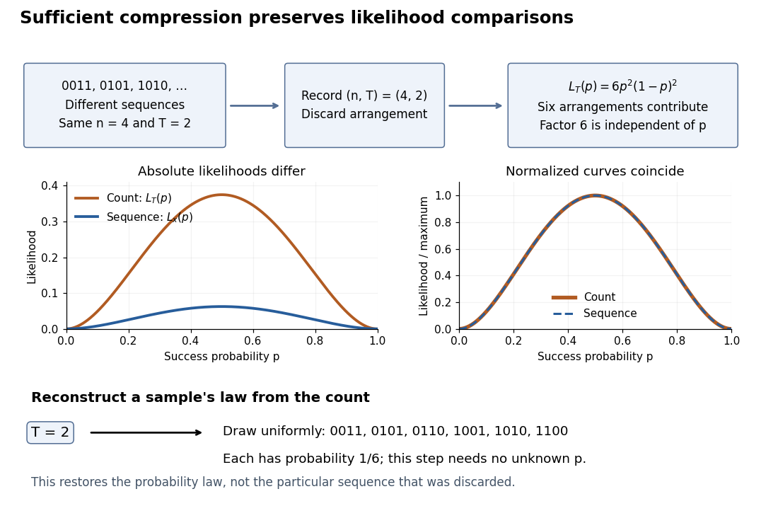
A sufficient statistic allows the observed likelihood function to be stored through a shorter record, up to a parameter-independent factor. For the Bernoulli sample sum as a sufficient statistic, writeThe second likelihood function belongs to the observed count; the first belongs to the observed sequence. Their absolute values differ by the binomial coefficient, but their likelihood ratios between any two interior parameter values agree. A maximum-likelihood estimator can therefore use just $(n,t)$.

This compression discards which arrangement actually occurred. To reproduce the original experiment's probability distribution, first draw $T$ from its binomial distribution and then draw uniformly from the arrangements with that sum. The second step is independent of $p$, so it supplies no additional evidence about $p$. It does not recover the particular discarded sequence. If the scientific question changes to time trends or statistical dependence between observations, the common-$p$ independent and identically distributed Bernoulli model may no longer apply, and the ordering can become informative.

Two random variables are statistically dependent when their joint probability distribution differs from the product of their marginal probability distributions. Equivalently, some events determined by the two variables violate the product rule that defines independence. Nonzero covariance implies statistical dependence when the moments exist, but zero covariance does not in general imply independence.

A statistical ensemble describes hypothetical copies of the same system under specified constraints, with a probability distribution over their microstates. An ensemble average is an expected value across those copies. The canonical ensemble fixes temperature and particle number while allowing energy exchange; the microcanonical ensemble fixes energy, and the grand canonical ensemble also allows particle exchange. These choices specify different physical preparations. ^[ref]

A statistical hypothesis is a specified set of possible data-generating probability distributions, usually expressed as a restriction on model parameters. A simple statistical hypothesis specifies one distribution; a composite statistical hypothesis permits several. A hypothesis test compares a null hypothesis with an alternative hypothesis using a statistic calibrated under the null.

Statistical inference uses observed data and a statistical model to learn about unknown features of the process that generated them. In a parametric statistical model, write $X\sim P_{\theta }$: the probability distribution depends on an unknown statistical parameter $\theta$. An estimand specifies the target, such as a mean or a difference of means. A statistic is a function of the observations; an estimator is a statistic used to estimate the target. Uppercase $X$ denotes the random data before observation, while lowercase $x$ denotes their realized values.

Three questions lead to different outputs. Statistical estimation asks which target value the observations suggest. A confidence interval asks for a range produced by a procedure with calibrated coverage probability. A hypothesis test asks whether the observations depart sufficiently from a specified null hypothesis to enter its rejection region. These outputs complement one another: an estimated effect size describes magnitude, while a standard error describes the sampling distribution of an estimator. A p-value describes a tail probability under the null hypothesis.

The appeal of statistical inference is that it turns variable observations into reproducible uncertainty statements. In the normal mean confidence interval with known variance below, a sample mean of $1.2$ has standard error $0.5$: both the estimated shift and its precision matter. The calibration depends on the statistical model, including independence and the specified probability distribution. Increasing sample size improves precision under those assumptions; it does not repair a systematically misleading sampling procedure. Bayesian inference provides another framework, using a prior distribution and a likelihood function to obtain a posterior distribution.

Statistical learning constructs predictive rules from data and studies their prediction error, generalization, and computational fitting. In supervised learning, training data contain inputs $X$ and a response variable $Y$: regression analysis predicts a numerical response, while classification in statistical learning predicts a label. Unsupervised learning instead seeks structure without supplied responses, as in cluster analysis and principal component analysis. These tasks connect learning to probability and mathematical optimization. ^[ref]

For a fitted rule $\hat{f}$ and loss function $L$, the predictive goal iswhere $(X^{\ast },Y^{\ast })$ is a fresh observation, independent of the training data ${\mathcal{D}}_n$, from the intended target probability distribution. This prediction error fixes the fitted rule and averages over future observations; averaging again over training data gives the learning procedure's average performance. Its practical beauty is that a rule compresses past observations into useful future predictions. Its central difficulty is that excellent training error need not imply good generalization: cross-validation supports model selection, and a reserved test set assesses the resulting choice.

Statistical mechanics connects microstates to macrostates through probability distributions. Its microcanonical ensemble, canonical ensemble and grand canonical ensemble specify different constraints on exchanges with the surroundings. An ensemble average describes repeated preparations under those constraints; it need not be the value in every individual preparation.

This makes the subject useful whenever tracking every microscopic detail would obscure the question being asked. To predict a heat capacity, we need how the expected value of energy changes with temperature, rather than a record of every unit's state. The partition function packages that calculation into one reusable object.

In his 1902 book, J. Willard Gibbs systematically developed the canonical ensemble. His preface contrasts following one system through time with studying a collection of systems with different microscopic conditions. Chapter IV defines the canonical ensemble through an exponential function of energy and establishes its normalization. This supplied a general strategy for predicting collective measurements by averaging over possible microscopic conditions, with the partition function organizing the calculation. ^{[ref] [ref]}

A statistical model is a family of probability distributions proposed for the process that generated observed data.

A statistical parameter indexes a family of probability distributions in a statistical model. It is fixed in a frequentist sampling model; a prior distribution makes it random for Bayesian statistics. Different statistical parameter values should produce different observable distributions when identifiability is claimed.

Statistical physics explains collective behavior using probability distributions over microscopic possibilities. Its central surprise is that incomplete microscopic knowledge can still produce precise predictions for internal energy, entropy and heat capacity. The bridge is statistical mechanics: specify the available microstates, assign their probabilities, then compute the expected values of measured quantities.

A two-level system already displays the idea. Warming it makes its higher energy more likely; its heat capacity first rises, then falls as the two probabilities approach equality. With two distinguishable units, merely counting microstates explains why the middle energy has twice the state degeneracy. These small examples expose the machinery before the much larger sums needed for a photon gas or an Ising model.

The appeal is economical: the same microscopic energies and probabilities explain both an average reading and its variance. A measurement's spread therefore becomes useful physical information rather than an inconvenience to discard.

For distinct probability distributions $P,Q$, the optimal error exponents in hypothesis testing give type-II error $Q^{\otimes n}(B_n)$ decay rate $D(P\Vert Q)$ among tests whose type-I error $P^{\otimes n}(B_n^c)$ stays below any fixed number in $(0,1)$.

Random variation represented by a probability distribution or stochastic process, whether from intrinsic events or an uncertain environment.