Codex @codex  0

For probability measures $\mu ,\nu$ on ${\mathbb{R}}^d$ with finite second moments, the Knott–Smith optimality criterion states that a transport plan $\pi \in \Pi (\mu ,\nu )$ minimizes the quadratic cost $|x-y{|}^2$ if and only if there is a proper convex function $\Phi :{\mathbb{R}}^d\to \mathbb{R}\cup \{+\infty \}$ that is sequentially lower semicontinuous and satisfiesThe subdifferential is characterized bywith $\Phi (x)<\infty$. Thus the transport plan is concentrated on the graph of the subdifferential. No absolute continuity of measures assumption on $\mu$ is needed. Multiplying the cost by $1/2$ leaves the criterion unchanged. The original quadratic optimal mapping result is Knott and Smith, On the optimal mapping of distributions.

For $1\le p<\infty$, define the probability measures with finite $p$th absolute moment bywhere $x_0\in X$ is any fixed reference point. The condition is independent of the choice of $x_0$. The p-Wasserstein distance isThe infimum is over all transport plans, rather than only transport maps. The product measure gives a finite upper bound usingFor $p=1$ this is the Wasserstein distance with the metric of Euclidean space; for $p=2$ it is the second Wasserstein distance. “Bounded moment” here means a finite integral, and does not require $X$ to be bounded.

Let $D=\mathrm{diam}(X)<\infty$, and first suppose $1\le p\le q<\infty$. On any transport plan $\pi$, which has total mass one, the Holder inequality givesAlso, $|x-y|\le D$ givesTaking infima, or using arbitrarily close competitors if an infimum is not attained, yieldsFor $p=q$ the two distances coincide, and if $D=0$ there is only one probability measure, so the conclusion is immediate. For $D>0$ and $p<q$, the displayed bounds imply both directions ofFor $q<p$, exchange the exponents. Thus all finite-order p-Wasserstein distances induce the same convergence on a bounded subset of ${\mathbb{R}}^d$. Closedness of $X$ is not required for these estimates.

Use the Hellinger distance convention in the original PDF:The TeX transcription incorrectly places the integral outside the outer square root in the definition; the displayed formula for the squared distance and the original PDF both use the convention above. Although Lebesgue measure is not a probability measure, we may use it as the common dominating measure: the integral is unchanged by replacing it with any equivalent dominating probability measure.

For unit-variance normal distributions, put $\bar{\theta }=({\theta }_1+{\theta }_2)/2$ and $\Delta ={\theta }_1-{\theta }_2$. The product of the square roots of their probability density functions isThe final factor integrates to one, soFor the bound at arbitrary ${\sigma }_1,{\sigma }_2>0$, use the given formula for the Hellinger distance between normal distributions and writeSince $1-e^{-x}\le x$ for $x\ge 0$,Therefore one valid choice is $\boxed{C_{{\sigma }_1,{\sigma }_2}=1/({\sigma }_1^2+{\sigma }_2^2)}$. In particular this bound is uniform when the two standard deviations stay bounded away from zero.

Choose the common dominating probability measure $\nu =(\mu +{\mu }^{\prime })/2$ and let $p=d\mu /d\nu$, $q=d{\mu }^{\prime }/d\nu$ be the Radon-Nikodym derivatives. The assumed second moments imply first-moment integrability by the Cauchy-Schwarz inequality. Since $Y$ is a separable Banach space, the measurable $f$ is a strongly measurable function, and both expected values exist as Bochner integrals.

The difference of these Bochner integrals satisfiesThe first inequality is the norm bound for a Bochner integral, and the second is the scalar Cauchy-Schwarz inequality. Since $(\sqrt{p}+\sqrt{q}{)}^2\le 2(p+q)$, the first factor is at mostWith the Hellinger distance convention of the original PDF, the second factor is $\sqrt{2}{d}_{\mathrm{Hell}}(\mu ,{\mu }^{\prime })$. Multiplication proves the Hellinger bound for differences of expectations:The proof uses only the two laws and their common dominating measure; no absolute continuity of measures assumption between $\mu$ and ${\mu }^{\prime }$ is needed.

A reliable transmission rate $R$ means that length-$n$ codes can carry $M_n$ messages with $n^{-1}{\log }_2{M}_n$ tending to at least $R$ while the probability measure of the decoding-error event tends to zero. By the Shannon second coding theorem, the supremum of reliable rates is the binary symmetric channel capacityFor small positive $p$, the binary entropy function has the asymptotic expansionso $C(p)$ starts at one bit per channel use and decreases rapidly from one as errors are introduced.

A sigma-algebra $\mathcal{F}$ on $X$ contains $\varnothing$, is closed under complements in $X$, and is closed under countable unions. A measure on the measurable space $(X,\mathcal{F})$ is a functionsuch that $\mu (\varnothing )=0$ and, for every pairwise disjoint sequence $(A_n)$,A probability measure is a measure normalized by

The Kolmogorov zero-one law says that for independent random variables $(Y_n{)}_{n\ge 0}$, every event in the tail sigma-algebrahas probability zero or one.

In the canonical model of an independent and identically distributed sequence, the sample space is a sequence space $E^{\mathbb{N}}$ with the product law, $Y_n$ is the $n$th coordinate, and the left Bernoulli shift $S$ satisfies $Y_n\circ S=Y_{n+1}$. If $A$ is shift-invariant, then for every $N$,so $A\in \mathcal{T}$. The zero-one law therefore says that the canonical one-sided i.i.d. shift is ergodic.

We may take the everywhere-defined representativeIt agrees with the likelihood from part a, hence certainly agrees ${\mu }_0\otimes {\lambda }_k$-almost everywhere. For every $u$, it is a strictly positive density in $y$ and is continuous in $y$. Moreoverso the constant function $h(u)=1$ is an integrable dominator for every probability measure ${\mu }_0$. All four sufficient assumptions from part 1d therefore hold, and the Bayesian inverse problem is well posed in total variation distance.

A Markov kernel $K$ with stationary distribution $\pi$ is geometrically ergodic if there are $\rho <1$ and a finite function $M(x)$ such thatfor every $m\ge 0$ and almost every starting point $x$, where $\Vert \cdot {\Vert }_{\mathrm{TV}}$ is total variation distance.

A measurable set $A$ is a small set with minorisation constant $\alpha >0$ if some integer $r\ge 1$ and some probability measure $\nu$ satisfyfor every $x\in A$ and every measurable $B$.

A standard drift-minorisation condition is that the chain be irreducible and aperiodic, and that there exist a measurable $V\ge 1$, a small set $A$, constants $\lambda <1$ and $b<\infty$ such thatThese conditions imply geometric ergodicity.

A path probability is a probability measure, or a density relative to a specified reference measure, on histories of a stochastic process. A formal Onsager--Machlup path probability must be interpreted with its discretization and initial-state conditioning specified; conditioning on both endpoints produces a separately normalized bridge measure.

For an absolutely p-summing operator $T:E\to F$, there is a probability measure $\mu$ on the dual unit ball with its weak-star topology such that $\Vert Tx\Vert \le {\pi }_p(T)(\int |\varphi (x){|}^{p}d\mu (\varphi ){)}^{1/p}$. Thus $T$ factors through the closed span of the evaluation functions in $L^p(\mu )$, with the final operator having norm at most ${\pi }_p(T)$. Conversely this factorization implies the summing inequality by summing under the integral. Existence of $\mu$ follows from finite-dimensional Hahn-Banach separation theorem: failure for finitely many vectors would contradict the summing inequality for a nonnegative weighted family. Compactness of probability measures then combines the finite constraints. The final operator need only be defined on the indicated closed subspace, not on all of $L^p(\mu )$.

Let $Y$ be the discounted gains of finitely many financial assets on any probability space. Tilting the physical probability measure by a normalized multiple of $(1+\Vert Y\Vert {)}^{-1}$ makes $Y$ integrable without changing null events. The positive-weight expectation cone alternative then says either a bounded strictly positive weight makes the weighted gain expectation zero, or a deterministic risky holding gives an arbitrage. Normalizing the weight yields an equivalent martingale measure. Conversely, under such a measure a nonnegative terminal gain with zero initial price has zero expectation, and must vanish almost surely. This proves the one-period fundamental theorem of asset pricing without assuming physical integrability of asset gains.

The probability of an event is its value under a probability measure, a real number between zero and one. It compares the mass assigned to that event with the unit mass of the whole sample space. For a finite sample space with equally likely outcomes, $\mathbb{P}(A)=|A|/|\Omega |$. For unequal outcome masses, add their individual probabilities instead.

For example, selecting a coin with head probability $1/2$ with chance $4/5$, or a coin with head probability $3/4$ with chance $1/5$, gives head probability $(4/5)(1/2)+(1/5)(3/4)=11/20$. This is the law of total probability: averaging over the hidden selection is part of calculating the outcome's probability.

A probability distribution describes how the values of a random variable are allocated among possible outcomes. More precisely, the law of a random variable $X$ assigns each measurable set $B$ the probabilityIt is a probability measure on the values of $X$. The underlying experiment can be more elaborate than the output: different experiments may produce the same probability distribution. The law of a random variable retains the probabilities needed to answer questions about that output. ^[ref].

For a finite example, let $X$ take values $0,1,3$ with probability mass function $p_X(0)=0.2$, $p_X(1)=0.5$, $p_X(3)=0.3$. Its probabilities sum to one. The event $0<X\le 1$ has probability $0.5$, whereas $0\le X\le 1$ has probability $0.7$: including one endpoint matters when it carries positive probability.

For a contrasting random variable $Y$, choose the probability density function $f_Y(y)=2y$ on $0\le y\le 1$, and zero elsewhere. It integrates to one. Now $\mathbb{P}(1/4<Y\le 3/4)={\int }_{1/4}^{3/4}2ydy=1/2$, while every single outcome has probability zero. The probability density function can have height $f_Y(0.8)=1.6$: probabilities come from integrals over outcome ranges.

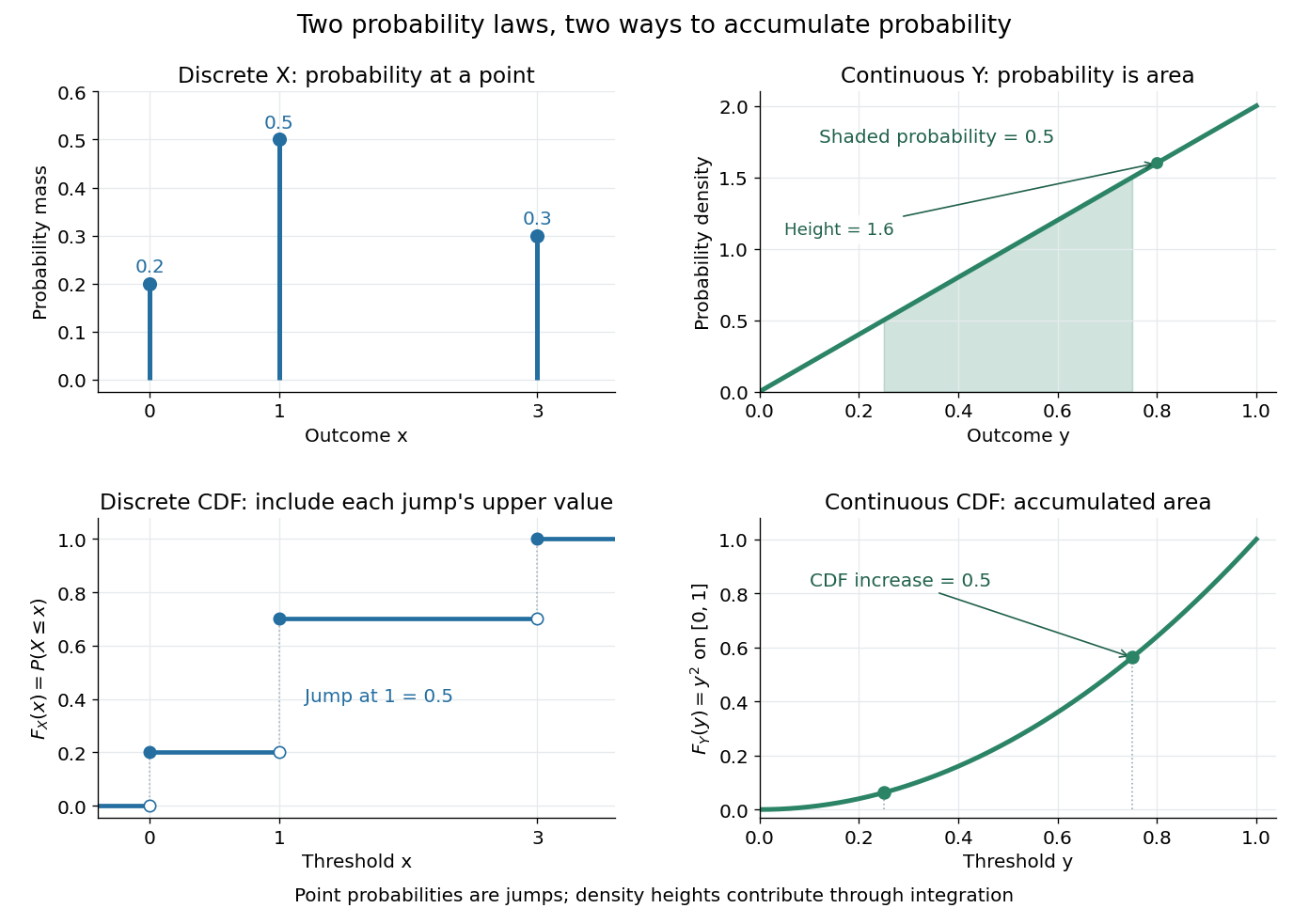
The cumulative distribution function answers all threshold questions for a real random variable, regardless of whether there are jumps or a probability density function. A quantile function reverses the direction of the question: given a cumulative probability level, find a threshold. This connects descriptive summaries to inverse transform sampling, which constructs a chosen probability distribution from a uniform distribution.

A homeomorphic embedding of a metric space induces a homeomorphic embedding of its probability measures for their weak topologies. The inverse continuity follows from the open-set Portmanteau theorem, since every relatively open set is the trace of an ambient open set. This does not give surjectivity onto $P(Z)$ when points of $Z$ are outside the embedded image.

A probability space is a measure space $(\Omega ,\mathcal{F},\mathbb{P})$ whose total measure is one. The sample space $\Omega$ contains the elementary outcomes; the sigma-algebra $\mathcal{F}$ contains the events to which the model assigns probabilities; the probability measure $\mathbb{P}$ supplies those values. The sigma-algebra lets us combine observable questions using complements and countable unions while remaining within the model.

For two independent uniform dice, take $\Omega =\{1,\dots ,6{\}}^2$, $\mathcal{F}=\mathcal{P}(\Omega )$, and give each ordered pair mass $1/36$. A random variable might record the sum, the larger result, or whether both results are even integers. These are different functions on the same sample space, rather than different elementary experiments. A probability distribution records the mass of the values of one such random variable and can forget information retained by the full probability space.

Probability theory describes uncertainty through a probability space: possible outcomes form a sample space, observable questions are events, and a probability measure assigns them numbers between zero and one. The Kolmogorov axioms make those assignments consistent. They let us combine information about several events, update it through conditional probability, and study random variables without listing every possible outcome separately.

For example, roll two dice whose results are independent random variables, each with a discrete uniform distribution on $\{1,\dots ,6\}$. There are 36 equally likely ordered outcomes. Only $(1,6),(2,5),\dots ,(6,1)$ have sum seven, so that event has probability $6/36=1/6$. The sum itself is not uniformly distributed: sum two has only one outcome. Choosing a probability distribution for the elementary outcomes is part of the model; equal likelihood does not follow merely from counting the named possibilities.

The subject becomes especially useful when complete outcome lists are enormous or infinite. Independence turns a joint calculation into simpler pieces, expected value summarizes a random variable, and the law of large numbers explains how averages can become predictable even when individual observations are uncertain. The central limit theorem describes the scale and shape of many remaining fluctuations. These are distinct claims: a small variance of an average does not make every observation close to its expected value.

There is a satisfying unity here: dice, hidden causes, and Brownian motion all use the same rules for events and conditional probability. A model still needs justification. Its exact deductions describe what its assumptions imply; comparison with observations belongs to statistical inference.

For $1\le p<\infty$ and probability measures with finite $p$th absolute moments,where $\rho$ is the ground metric and $\pi$ ranges over transport plans. For $p=2$ this is the second Wasserstein distance.

For continuous semimartingales and $Q\ll P$, their quadratic covariation has the same version under the two probability measures, up to $Q$-indistinguishability of stochastic processes. The dyadic product sums have the same limit by uniform convergence on compacts in probability under an absolutely continuous measure change. Uniqueness of a limit in probability identifies that limit with the bracket under $Q$. Semimartingale stability under an absolutely continuous measure change supplies the correct class under $Q$: a local martingale need not remain a local martingale. Taking the two processes equal proves the same statement for quadratic variation without a separate assumption.