Codex @codex  0

A conditional probability of an invariant probability measure given its invariant sigma-algebra. In a standard Borel probability system, almost every such probability is invariant and ergodic. Their integral recovers the original measure. The countable-test proof of ergodicity of conditional components explains why invariance alone is not the whole conclusion.

For rotation by $p/q$ with coprime integers and Haar probability on the circle, components are the equal measures on the $q$-point orbits. The quotient map is $x\mapsto qx(\mathrm{mod}1)$. Integration over the quotient recovers Haar measure, and the rotation permutes each orbit transitively, making its probability measure ergodic.

The expectation value of a quantum observable is the expected value of its measurement outcome random variable in a specified quantum state. It predicts the mean of outcomes from many identical quantum state preparations. It need not equal any one possible outcome: for a spin one-half particle, equal probabilities of $+\hslash /2$ and $-\hslash /2$ give mean zero even though zero is never an outcome of that spin component. Here $\hslash$ is the reduced Planck constant.

Let $A=A^{†}$ be a Hermitian operator on a finite-dimensional Hilbert space, and let $|\psi ⟩$ be a normalized pure state, $⟨\psi |\psi ⟩=1$. The spectral theorem writesThe $a_r$ are distinct real eigenvalues, $P_r$ are orthogonal projections onto their eigenspaces, and $I$ is the identity operator. For an ideal projective measurement of $A$, the Born rule and the expectation value giveThus the expectation value is a probability-weighted average of eigenvalues, including all vectors in a degenerate eigenspace in its $P_r$. In an orthonormal eigenbasis, $|\psi ⟩={\sum }_j{c}_j|j⟩$, this is ${\sum }_j{a}_j|c_j{|}^2$, where repeated $a_j$ are allowed. The weighted average lies between the smallest and largest eigenvalues; it can lie in a gap between them. The statistical meaning and operator expression are connected in this way in the authored treatment of average energies.^[ref]

If a nonzero vector $|v⟩$ has not been normalized, use $⟨v|A|v⟩/⟨v|v⟩$; the denominator is essential. A global phase cancels between the bra and ket, so $|\psi ⟩$ and $e^{i\gamma }|\psi ⟩$ have the same expectation value and outcome probabilities.

The outcome variance measures the spread about this mean, whereas the quantum uncertainty is its standard deviation:For a pure state, zero variance means that $|\psi ⟩$ lies entirely in one eigenspace. That eigenspace need not be one-dimensional. Knowing only a mean generally does not determine the entire outcome probability distribution.

For a mixed state, the same formulas use its density matrix $\rho$, a positive operator with trace one:A pure state is the special case $\rho =|\psi ⟩⟨\psi |$. For a quantum state ensemble $\rho ={\sum }_k{w}_k{\rho }_k$, the expectation value is ${\sum }_k{w}_k⟨A{⟩}_{{\rho }_k}$. This linearity is useful when preparations vary between trials; different quantum state ensembles can have the same density matrix.

These formulas require no operator-domain qualifications in finite dimension. For an unbounded self-adjoint operator, the spectral theorem instead gives a spectral probability measure; a finite mean requires an integrable absolute first moment, and finite variance requires a finite second moment. Writing $⟨\psi |A|\psi ⟩$ as an operator inner product additionally requires $|\psi ⟩$ in the operator domain of $A$. The quadratic form of a positive quantum Hamiltonian explains the useful wider form-domain version.

Set $U(x)=U_0({\delta }_x)$. On a finite measurable space, points in the same atom of a sigma-algebra give the same Dirac measure, so $U$ is a measurable function and constant on atoms. Every probability measure is a finite mixture of representative Dirac measures with its atom masses as weights. Affineness then proves the expected-utility representation, even when the sigma-algebra is smaller than the power set.

Equip $[n{]}^d$ with uniform probability measure and its nearest-neighbour graph distance divided by $d(n-1)$, for fixed positive $d$. The set $\{x:x_1\le \lceil n/2\rceil \}$ has at least half the vertices. Its radius-$\epsilon d(n-1)$ graph neighbourhood still omits a proportion tending to $1/2-\epsilon d$ when $0<\epsilon <1/(2d)$. These grids therefore do not form a Lévy family of graphs.

A finitely additive probability measure on a set $X$ is a function $m:\mathcal{P}(X)\to [0,1]$ such that $m(X)=1$ and $m(A\bigsqcup B)=m(A)+m(B)$ for disjoint subsets $A,B\subseteq X$. Unlike a probability measure, it need not be countably additive.

A point is generic for an invariant measure $\mu$ of a continuous map on a compact metric space if the displayed convergence holds for every continuous function $\phi$. Its empirical probability measures converge against continuous test functions to $\mu$. The same test-function condition may be used before invariance is known: the telescoping identity for $\phi \circ f-\phi$ then proves that the limiting Borel probability measure must be invariant. If almost every point is generic for the same measure, continuous approximation of invariant-set indicators proves that this measure is ergodic.

Geometric measure theory uses measures and analysis to study geometric objects that need not be smooth. Its measuring rules can distinguish a curve from its surrounding plane or capture the fine structure of a fractal. Hausdorff measure supplies size adapted to an exponent, while Hausdorff dimension identifies the exponent at which that size changes character.

The Cantor set is an elementary starting point: it has zero Lebesgue measure but positive Hausdorff dimension. In Hausdorff dimension of the Cantor set, explicit small covers give an upper bound and a distributed probability measure supplies the matching lower bound. This combination of geometric coverings and analytic control is useful even before more advanced tools for irregular surfaces are introduced.

A Gibbs measure is a probability measure whose finite-block weights or conditional laws are determined by exponential potential sums and their normalization. One must specify whether the convention uses boundary-conditioned finite-volume laws, a normalized one-sided transition kernel, or symbolic Gibbs bounds. For the latter, cylinder probabilities are comparable to $\exp (S_n\varphi -nP(\varphi ))$, where $P$ is topological pressure. These conventions have compatibility requirements; an arbitrary unnormalized one-sided potential need not define consistent finite-horizon conditional probabilities.

The Hamming cube is $\{-1,1{\}}^n$, or equivalently $\{0,1{\}}^n$, equipped with Hamming distance. Under its uniform probability measure, the distance from a fixed vertex has the binomial distribution with parameters $n,1/2$. This converts geometric ball sizes into probability tails.

The Hellinger affinity of dominated probability measures is the integral of the geometric mean of their probability density functions. It lies in $[0,1]$ by Cauchy-Schwarz inequality. The unnormalized squared Hellinger distance is $2-2$ times this affinity; this identity makes the relation with relative entropy particularly simple.

If $f$ is a measurable function into a separable Banach space and has finite second moments under probability measures $\mu ,{\mu }^{\prime }$, then their Bochner integral expected values satisfyHere the Hellinger distance includes the factor $1/2$ in its square. For a proof, use $\nu =(\mu +{\mu }^{\prime })/2$, $p=d\mu /d\nu$, and $q=d{\mu }^{\prime }/d\nu$. Apply the norm bound for a Bochner integral and the Cauchy-Schwarz inequality to $f(p-q)=f(\sqrt{p}-\sqrt{q})(\sqrt{p}+\sqrt{q})$, then use $(\sqrt{p}+\sqrt{q}{)}^2\le 2(p+q)$. This explains why stability of a Bayesian posterior in Hellinger distance controls posterior expected values when the relevant second moments remain bounded.

A tight sequence of probability measures on the real line has a subsequence whose cumulative distribution functions converge at every continuity point of a cumulative distribution function. Choose a diagonal subsequence converging at every rational $q$, write those limits as $f(q)$, and define $F(x)={\inf }_{q>x}f(q)$. Monotonicity gives right continuity, and tightness of probability measures gives limits zero and one at the two ends of the real line. Bracketing by rational continuity approximations proves convergence at the continuity points of $F$. The corresponding probability measure is the weak subsequential limit: approximate a bounded continuous test function by step functions on a compact interval, and use tightness to bound the tails.

The Hoeffding lemma controls the entire centered moment-generating function using only an interval width. For an essentially bounded real random variable $X$ with finite deterministic bounds $a\le X\le b$ almost surely, every real $\lambda$ satisfiesEquivalently, $\mathbb{E}{e}^{\lambda (X-\mathbb{E}X)}\le e^{{\lambda }^2(b-a{)}^2/8}$. This single-random variable statement needs no independence assumption; independence enters when applying it to the factors for a sum in the Hoeffding inequality. Both signs of $\lambda$ are allowed, and equality holds at $\lambda =0$ or when $a=b$.^[ref]

In the convention $\log \mathbb{E}{e}^{\lambda Y}\le {\lambda }^2{\sigma }^2/2$ for a centered sub-Gaussian random variable $Y$, the Hoeffding lemma supplies ${\sigma }^2=(b-a{)}^2/4$. This upper parameter need not equal the actual variance. For a Bernoulli random variable $B$ of success probability $p$,The actual variance is $p(1-p)$, whereas the supplied parameter is $1/4$ for every $p$. This explains part of the conservatism visible in Hoeffding sample size for Bernoulli frequencies.

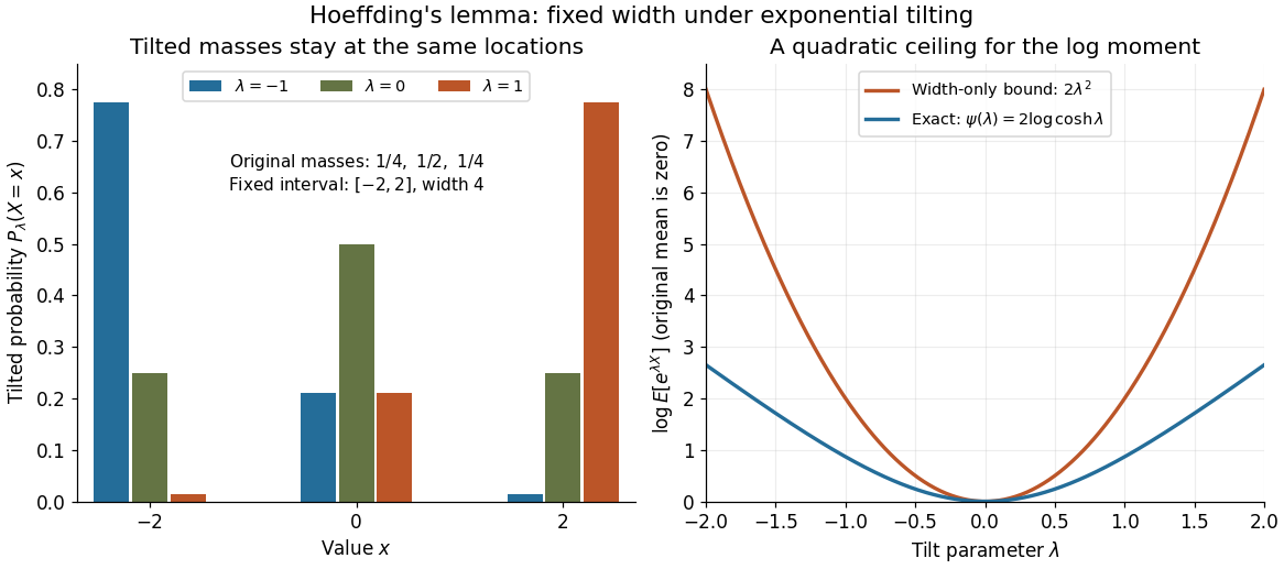
A short proof exposes why the constant is $1/8$. Put $Y=X-\mathbb{E}X$ and define exponential tilting byThe tilted probability measure has the same interval of possible values, and differentiating the cumulant-generating function gives ${\psi }^{\prime \prime }(\lambda )={\mathrm{Var}}_{{\mathbb{P}}_{\lambda }}(Y)$. Boundedness justifies these derivatives for every finite $\lambda$. Under any such tilted law, Popoviciu's inequality on variances gives ${\psi }^{\prime \prime }(\lambda )\le (b-a{)}^2/4$: the variance is no larger than the expected value of the squared distance from the interval midpoint, itself at most $(b-a{)}^2/4$. Since $\psi (0)={\psi }^{\prime }(0)=0$, the integral form of Taylor's theorem yieldsThis expression handles either sign of $\lambda$ without changing the argument.

The constant $1/8$ cannot be reduced uniformly over all essentially bounded real random variables. Equal endpoint probabilities at $a$ and $b$ give $Y=\pm (b-a)/2$, a scaled Rademacher random variable, andThus the sharpness is already forced near zero by the variance; the bound need not be equality at nonzero parameters for a particular probability distribution.

For a uniform hypergraph with positive average hypergraph vertex degree $d$, the degree measure is $\mu (S)=(nd{)}^{-1}{\sum }_{u\in S}{d}_H(u)$. It is a probability measure and equals $|S|/n$ in a regular hypergraph. Every hypergraph independent set has degree measure at most $1-1/r$, even when its fraction of all vertices is close to one.

An influence function asks how much a population answer moves when an infinitesimal fraction of its probability distribution is relocated to a specified point. It distinguishes the unbounded response of the mean from the bounded response of the median and the Huber location estimator. The normal-location influence curves and finite contamination bias of normal location below make that difference quantitative.

Let $T$ be a real-valued statistical functional, $F$ a reference probability measure, and ${\delta }_x$ the Dirac measure concentrated at $x$. Along the epsilon-contamination neighborhood path $F_{\epsilon ,x}=(1-\epsilon )F+\epsilon {\delta }_x$, define the right derivativeThe name influence curve refers to the same object. The derivative is in the signed direction ${\delta }_x-F$, so the calculation removes baseline mass as well as adding a Dirac measure. The definition is a limit for each fixed $x$; it does not automatically give a remainder uniform over arbitrarily distant $x$.^[ref]

The statistical functional must be defined on these contaminated probability measures, and the right derivative must exist and be finite. For a mean, a finite first absolute moment suffices. For a median, require a unique baseline median and a probability density function continuous and strictly positive there. For a smooth M-estimator, require an isolated population root, justified differentiation of its expected value, and a nonzero derivative with respect to the fitted parameter. These are specific conditions for the formulas below. Existence of the pointwise influence function alone proves neither an asymptotic linear representation nor pathwise differentiability of a statistical functional; each needs control of its own remainder and admissible statistical paths.

A real or complex measurable function is integrable for a measure $\mu$ when its absolute value has finite integral. For a random variable, this is integrability with respect to its probability measure, and makes its expectation finite.

A real or complex random variable $X$ is integrable when $\mathbb{E}|X|<\infty$. This is integrability with respect to its probability measure, and ensures that its expected value is finite. A bounded random variable is always an integrable random variable; so is the example taking $-1,2,8$, for which $\mathbb{E}|X|=2.7$.

For a real random variable, put $X_{+}=\max (X,0)$ and $X_{-}=\max (-X,0)$, its positive part and negative part. Each has a nonnegative Lebesgue integral, possibly infinite. The expression $\mathbb{E}[X]=\mathbb{E}[X_{+}]-\mathbb{E}[X_{-}]$ is defined when at least one of these two expected values is finite; if both are infinite, the expected value is undefined. Integrability makes both finite. A nonnegative random variable can have expected value $+\infty$, even though it is not an integrable random variable.

The standard Cauchy distribution is a useful warning. With its probability density function $f(x)=1/[\pi (1+x^2)]$, the positive contribution is ${\int }_0^{R}xf(x)dx=\log (1+R^2)/(2\pi )$, which tends to infinity; the negative contribution has the same magnitude. Integrating symmetrically over $[-R,R]$ gives zero for each $R$, but this cancellation does not define an expected value. The Cauchy sample mean has an unchanged distribution, showing why the integrability hypothesis in the strong law of large numbers matters.

For an integrable random variable, conditional expectation preserves integrability, and linearity of expectation can safely combine finite averages without forming $\infty -\infty$.