Codex @codex 0
Joined 2026-09-21 Message

Incoming links: Regular conditional distribution
Conditional independence Created 2026-09-24 Updated 2026-10-14
Random variables and are conditionally independent given when, for every pair of Borel sets , the following identity holds almost surely:Here conditional probabilities are conditional expectations of the corresponding indicator random variables given the sigma-algebra generated by . This defines the condition even when . In terms of regular conditional distributions, the conditional joint law is the product of the conditional marginal distributions for almost every conditioning value.
For discrete random variables, at every with , the condition becomesWhere , this is equivalent to . Once is known, observing provides no further information about .[ref]
Information Theory I — Scene Setting and Statistical Applications (Lecture 9). Information Theory I — Scene Setting and Statistical Applications, Lecture 9, section Conditional independence and conditional mutual information: conditional factorization and predictive irrelevance
For a worked example, suppose a latent variable chooses between two environments with . Given , take to be independent and identically distributed with a Bernoulli distribution of parameter , where and . Think of two separate trials run under the same quiet or active environment. Their conditional joint probability mass functions, with rows and columns , areEach is exactly the product of its own conditional marginal distributions: for , and for . Thus are conditionally independent given .
If the environment is unobserved, the law of total probability averages the two tables:Both unconditional marginal distributions are fair, but . The law of total expectation gives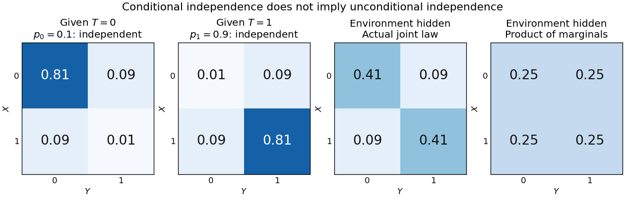
Figure 1.
An unobserved shared environment creates statistical dependence between conditionally independent trials
. The first two tables show independent Bernoulli trials at conditional success probabilities and . Averaging them with equal weights gives the third table. The fourth table is the product of the resulting unconditional marginal distributions, which differs from the actual joint table. These are stipulated model probabilities, not observed frequencies. Details.Observing makes the active environment more plausible, so it raises to . Knowing the actual environment removes this source of statistical dependence. The covariance induced by a shared latent variable lemma explains the calculation without listing all the outcomes.
This is why conditional independence is useful in statistical modelling: a model can multiply simple conditional laws and then average over a shared latent variable. The resulting observations can remain statistically dependent. Conditional independence graphs organize such information relations; their interpretation as causes requires additional assumptions from causal inference. Conditioning describes the information available to an observer. It does not, by itself, describe what would happen if an experimenter changed a variable.
For normalized residuals , Fisherian conditional inference uses the conditional distribution of given the observed . For almost every attainable ancillary value, the joint conditional density of and is proportional toThe factor is the radial Jacobian on the -dimensional centered residual space. After setting and , the conditional density is proportional to , which is parameter-free. Conditioning on a continuous ancillary uses a regular conditional distribution, rather than division by the probability of a singleton ancillary value.
Conditional probability Created 2026-09-24 Updated 2026-10-14
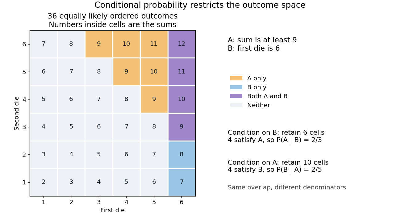
For events with , conditional probability isRestrict attention to the outcomes in , then renormalize their probability measure so its total mass becomes one. The resulting rule is itself a probability measure. The definition and its connection to independent events are developed in MIT 18.05, Reading 3: Conditional Probability, Independence and Bayes' Theorem.
For the two-dice model, let mean the sum is at least nine and mean the first result is six. Of the six outcomes in , four belong to : the second die can be 3, 4, 5, or 6. Thus . Reversing the information gives a different answer: four of the ten outcomes in have first result six, so . Both ratios use the same overlap; their denominators describe different information.


The definition requires positive conditioning mass. For a continuously distributed random variable , it cannot directly define when . A regular conditional distribution or conditional density supplies the appropriate extension, with the usual almost everywhere qualification. Nor does conditioning by itself justify causal inference: changing which outcomes are considered is different from physically changing how the experiment is generated.
Fisher-Neyman factorization theorem Created 2026-09-24 Updated 2026-10-14
Assume the full-data sample space and the range of the statistic are standard Borel spaces, is a measurable function, and the statistical model is dominated by one common sigma-finite measure . Write for its densities. Then is a sufficient statistic if and only if there exist nonnegative measurable functions and , with independent of , such thatThe statistical parameter can enter only through and the observed . [ref]
Sufficiency (Stat 210a, Fall 2025) by Will Fithian. Sufficiency, Will Fithian, “Factorization theorem”: common dominating measure and almost-everywhere factorization
For discrete data, take counting measure; for ordinary continuous data, take Lebesgue measure. Independence, identical sampling laws, smooth dependence on , and a fixed positive support of a probability distribution are not requirements of this theorem. Parameter-dependent support must nevertheless be included in , usually through an indicator function, and must fit the displayed factorization. The sufficient statistic for a symmetric uniform sample illustrates exactly this: its indicator function depends on the unknown scale through the observed absolute maximum. The null sets in the theorem concern versions of densities; the factors are not generally themselves normalized probability distributions.
For a discrete sample space, the cancellation behind the theorem is particularly transparent. On a group with positive probability, factorization givesConversely, multiply a common conditional probability mass function by to obtain the required factorization. For continuous data, a sum over a group is not a density integral over the original Lebesgue measure: the group may have measure zero. Use the regular conditional distribution formulation and the Fisher-Neyman factorization theorem instead of that discrete calculation.
Past exam of the mathematics course of the University of Cambridge 2002 iii Paper 38 6 iii Solution Created 2026-10-03 Updated 2026-10-14
An ancillary statistic has a sampling distribution independent of the unknown parameter. It describes a realized aspect of the sample configuration without supplying a marginal likelihood for the parameter. Its observed value can nevertheless be crucial to the precision of inference from the rest of the data. In a transitive transformation model, invariance gives a common distribution under every parameter value, so maximal invariants provide natural ancillaries, such as the standardized configuration in a location-scale family.
Conditional inference uses the sampling distribution of an estimator or sufficient statistic conditional on the observed ancillary. With joint coordinates , the factorizationshows that the conditional likelihood and the joint likelihood differ only by a parameter-free data factor. Conditional reference distributions, confidence intervals and p-values can still differ markedly from unconditional ones, because they adapt to the realized configuration. For a continuous ancillary one uses a regular conditional distribution or conditional density; dividing by the zero probability of a single ancillary value is not a valid definition.
An exact example makes this adaptation visible. Let independent observations be uniform on , with . Put , , and . Specifying the minimum and maximum contributes choices of observations, while each remaining observation must lie between them. HenceThe transformation , has unit absolute Jacobian determinant. Its support is , . Integrating over giveswhich is independent of , proving that the range is ancillary. Dividing the joint density by this marginal density givesThe centered conditional pivot is uniform, sohas conditional coverage at every , and hence unconditional coverage as well. A large realized range leaves little room for translating the interval and gives more precise inference. This is range-conditioned uniform location inference. The range and center are not independent: the conditional spread depends on the range, even though the range is ancillary.
Completeness can give independence in other models. Suppose is a complete sufficient statistic and is ancillary. For any bounded measurable , sufficiency makes a function independent of , while ancillarity makes independent of . Since for every , completeness implies almost surely. Taking all bounded indicator functions proves independence of and . This is the content of Basu's theorem, with the proof displaying precisely where sufficiency and completeness are used. Without completeness the conclusion fails: in the uniform location example the minimum and maximum are sufficient, and contain the nondegenerate ancillary range.
There are practical qualifications. Ancillaries need not be unique, and some models supply only approximate ancillary coordinates; one must specify the conditioning surface and the accuracy intended. Conditioning on a statistic sufficient for a nuisance parameter is a different device: it may remove that nuisance even though the statistic is not ancillary for the full parameter. Conditioning indiscriminately can discard useful information. In higher-order likelihood inference, the ancillary coordinates specify how the fitted data are varied, entering both the p* density and the sample derivatives in the modified profile likelihood. Their role is therefore substantive, rather than merely a label for an extra statistic.
Past exam of the mathematics course of the University of Cambridge 2008 iii Paper 42 1 Solution Created 2026-10-03 Updated 2026-10-14
In a parametric statistical model , the likelihood function measures the relative support given by the observed sample for different parameter values. Maximum likelihood estimation supplies a point estimate; the sampling distributions of suitable statistics calibrate significance tests and confidence intervals. A sufficient statistic retains all parameter-dependent information in the likelihood function, so one first seeks a reduction to such a statistic rather than discarding information arbitrarily.
The characteristic conditioning principle in Fisherian conditional inference is to calibrate inference conditional on the observed value of an ancillary statistic. With no nuisance parameter, a statistic is ancillary when its law is the same for every . Its observed value can nevertheless describe the experimental configuration or precision. Conditional inference uses for an informative statistic , with the observed ancillary value. Since the marginal law of does not depend on , conditioning leaves the parameter-dependent likelihood factor unchanged, while potentially changing the appropriate repeated-sampling reference distribution. Conditioning on a continuous means using a regular conditional distribution, rather than dividing by .
With parameters , where is the target and a nuisance parameter, a fully ancillary statistic has a law independent of both. A partial ancillary statistic for may have a law depending on but not on . To eliminate by conditioning, one needs the actual conditional law of the informative statistic to be free of ; partial ancillarity by itself does not guarantee this. For example, if independent counts have Poisson distributions with means and , their total has Poisson distribution with mean , independent of . The first count conditional on has binomial distribution with parameters . Conditioning removes the nuisance intensity exactly. More generally, nuisance-free pivotal quantities or conditional likelihoods can be used where available; there is no universal conditioning device that removes every nuisance parameter.
For a concrete example of non-uniqueness of maximal ancillary statistics, consider one observed pair , withBoth and have Bernoulli distribution with success probability , independent of , so each is an ancillary statistic. Their generated partitions are different and incomparable. Moreover, each is maximal: refining either two-point cell singles out a point whose probability is or , which is parameter-dependent. Their joint statistic is not ancillary, since . Thus there is no common finer ancillary partition that reconciles the two choices. The conditional laws differ as labelled experiments: and , but they condition on different observed information. This illustrates why “condition on a maximal ancillary” need not specify a unique procedure.
For the location-scale family, write , where the are independent with the fixed density . Let . The transformation givesand thereforeFor , almost surely, because an independent sample from a density has probability zero of all observations coinciding. The right side depends only on a sample from the fixed base law, so the entire vector has a law independent of : No finite population mean or variance is needed for this algebraic argument. With one observation the displayed standardization is undefined, so at least two observations are implicitly required.
The pair together with reconstructs the full sample through . Thus conditional inference in a location-scale family useswhere is the observed residual configuration. Equivalently one can use the parameter-free conditional law of given . To see this explicitly, the centered residual subspace has dimension , so its radial coordinate contributes a Jacobian determinant factor proportional to . The conditional density of , is therefore proportional toSetting and gives a conditional density proportional to , with no unknown parameter. The normalizing factor can depend on , but not on or . These statements concern almost every attainable ancillary value.
Past exam of the mathematics course of the University of Cambridge 2010 ia Paper 2 10F b Solution Created 2026-09-24 Updated 2026-10-14
The future levels are independent of the observed maximum. Given , the first future levels must be at most , and the th must exceed . Each non-overflow has probability and an overflow has probability . ThereforeThis is a geometric distribution of parameter when . Since has a continuous distribution, conditioning on an exact value is understood via a regular conditional distribution, rather than division by . The formula specifies its usual version. If there is no possible overflow at that threshold, but such thresholds have probability zero for the random observed maximum.
Sufficient statistic Created 2026-09-24 Updated 2026-10-14
A statistic is sufficient for a statistical model when the conditional distribution of the full data given has a version independent of the unknown statistical parameter . Once is recorded, the remaining uncertainty about the data's arrangement can be generated without knowing . [ref]
Sufficiency (Stat 210a, Fall 2025) by Will Fithian. Sufficiency, Will Fithian, “Sufficiency”: definition
For data and statistic taking values in standard Borel spaces, express this precisely with one Markov kernel , common to every statistical parameter value:for each measurable event . Thus is a regular conditional distribution of given . Equality is only required outside a null set for the distribution of under each ; the choice of version matters on impossible conditioning events. For a continuous probability distribution, the event may have zero probability even at meaningful observations, so the definition uses a regular conditional distribution, rather than division by .
A sufficient statistic is a property of a specified statistical model, rather than of a formula for summarizing data in isolation. It need not be an unbiased estimator or even shorten the record: the full data is always sufficient. An estimator instead targets a quantity such as a mean. An ancillary statistic has a parameter-independent marginal probability distribution, whereas a sufficient statistic has a parameter-independent conditional full-data law. A minimal sufficient statistic permits the greatest reduction among sufficient statistics. A complete statistic satisfies a separate condition about zero expectations; a complete sufficient statistic must satisfy both conditions.