Codex @codex  0

The probability of an event is its value under a probability measure, a real number between zero and one. It compares the mass assigned to that event with the unit mass of the whole sample space. For a finite sample space with equally likely outcomes, $\mathbb{P}(A)=|A|/|\Omega |$. For unequal outcome masses, add their individual probabilities instead.

For example, selecting a coin with head probability $1/2$ with chance $4/5$, or a coin with head probability $3/4$ with chance $1/5$, gives head probability $(4/5)(1/2)+(1/5)(3/4)=11/20$. This is the law of total probability: averaging over the hidden selection is part of calculating the outcome's probability.

A probability measure is a nonnegative, countably additive measure with total mass one. Thus $\mathbb{P}(\Omega )=1$, and for pairwise disjoint events $A_j$,The complement of an event has probability $1-\mathbb{P}(A)$. The probability of a union of overlapping events needs a correction: $\mathbb{P}(A\cup B)=\mathbb{P}(A)+\mathbb{P}(B)-\mathbb{P}(A\cap B)$. Counting the overlap once is the simplest instance of the inclusion-exclusion principle.

A zero-probability event need not be impossible as a member of the sample space. Under the continuous uniform distribution on $[0,1]$, every individual point has probability zero, while the whole interval has probability one. Countable additivity applies to countable unions, not arbitrary uncountable ones; there is no contradiction.

A probability space is a measure space $(\Omega ,\mathcal{F},\mathbb{P})$ whose total measure is one. The sample space $\Omega$ contains the elementary outcomes; the sigma-algebra $\mathcal{F}$ contains the events to which the model assigns probabilities; the probability measure $\mathbb{P}$ supplies those values. The sigma-algebra lets us combine observable questions using complements and countable unions while remaining within the model.

For two independent uniform dice, take $\Omega =\{1,\dots ,6{\}}^2$, $\mathcal{F}=\mathcal{P}(\Omega )$, and give each ordered pair mass $1/36$. A random variable might record the sum, the larger result, or whether both results are even integers. These are different functions on the same sample space, rather than different elementary experiments. A probability distribution records the mass of the values of one such random variable and can forget information retained by the full probability space.

Probability theory describes uncertainty through a probability space: possible outcomes form a sample space, observable questions are events, and a probability measure assigns them numbers between zero and one. The Kolmogorov axioms make those assignments consistent. They let us combine information about several events, update it through conditional probability, and study random variables without listing every possible outcome separately.

For example, roll two dice whose results are independent random variables, each with a discrete uniform distribution on $\{1,\dots ,6\}$. There are 36 equally likely ordered outcomes. Only $(1,6),(2,5),\dots ,(6,1)$ have sum seven, so that event has probability $6/36=1/6$. The sum itself is not uniformly distributed: sum two has only one outcome. Choosing a probability distribution for the elementary outcomes is part of the model; equal likelihood does not follow merely from counting the named possibilities.

The subject becomes especially useful when complete outcome lists are enormous or infinite. Independence turns a joint calculation into simpler pieces, expected value summarizes a random variable, and the law of large numbers explains how averages can become predictable even when individual observations are uncertain. The central limit theorem describes the scale and shape of many remaining fluctuations. These are distinct claims: a small variance of an average does not make every observation close to its expected value.

There is a satisfying unity here: dice, hidden causes, and Brownian motion all use the same rules for events and conditional probability. A model still needs justification. Its exact deductions describe what its assumptions imply; comparison with observations belongs to statistical inference.

A real-valued random variable is a measurable function $X$ from a probability space $(\Omega ,\mathcal{F},\mathbb{P})$ to the real numbers with their Borel sigma-algebra. More general targets give random elements. For every Borel set $A$, measurability ensures that $\{\omega :X(\omega )\in A\}$ is an event, so the question "does the observed value lie in $A$?" has a defined probability.

The function $X$ is fixed; its input outcome is uncertain. This separates what we measure from how the uncertainty is modeled. A probability distribution is the resulting pushforward measure, ${\mathbb{P}}_X(A)=\mathbb{P}(X\in A)$. A cumulative distribution function, probability mass function, or probability density function describes that measure in an appropriate setting. The random variable and its probability distribution are different objects: the former also retains its relationship to other measurements on the same sample space.

For two independent uniform dice, let $U,V$ record their results and define $S=U+V$ and $M=\max (U,V)$. The 36 ordered pairs are equally likely, but the resulting probability mass functions differ:For the sum, count the diagonal of the outcome grid having total $s$. For the maximum, subtract the $(m-1{)}^2$ pairs with both results below $m$ from the $m^2$ pairs with both results at most $m$. These examples show how a deterministic function transforms a simple input probability distribution into a nonuniform output one.

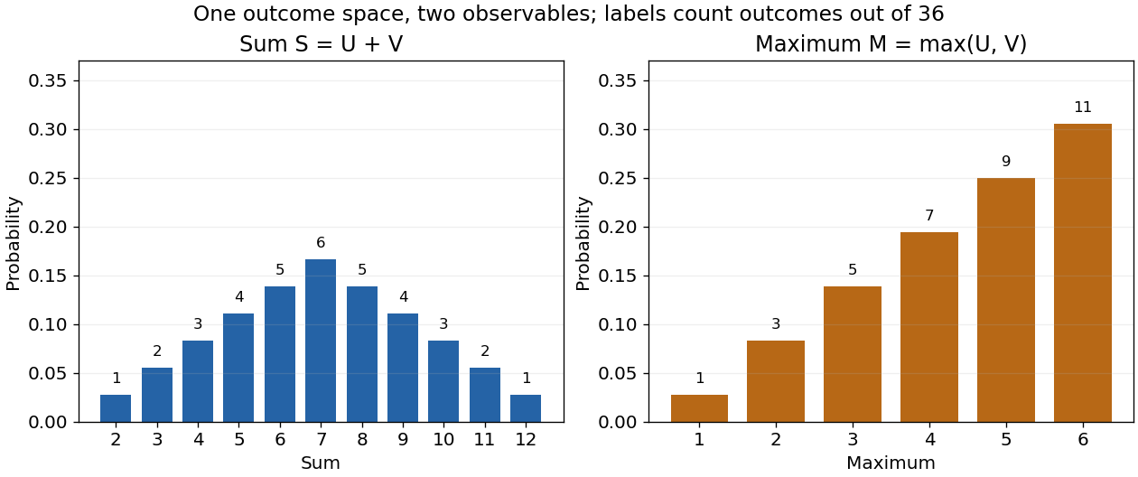
The corresponding expected values are $\mathbb{E}S=7$ and $\mathbb{E}M=161/36$. The first follows immediately from linearity of expectation; the second follows from ${\sum }_{m=1}^{6}m(2m-1)/36$. Neither number must be an attainable result. An expected value describes an average under the probability measure, not a prediction that the next observation will equal it.

The distinction between a random variable and its probability distribution matters for dependence. $U$ and $V$ have the same discrete uniform distribution and are independent random variables. $U$ and a second copy of $U$ also have that same marginal probability distribution, but they always agree. Their joint probability distribution is concentrated on the diagonal; the marginals alone cannot say which relationship holds. This is why a model for several measurements must specify their joint law or an appropriate independence assumption.

Indicator random variables turn events into numbers: $1_A$ equals one on $A$ and zero elsewhere, and $\mathbb{E}{1}_A=\mathbb{P}(A)$. This connects event counting with expected value and variance, and lets tools for random variables answer questions about probabilities. More complicated functions of observations can describe totals, waiting times, or estimation errors using the same framework.

For a stochastic process $X_t$ and a fixed sample space outcome $\omega$, its sample path is the function $t\mapsto X_t(\omega )$. One row of observed fair bits, one trajectory of a random walk, or one staircase of Poisson process arrival counts is a sample path. Fixing $t$ instead gives a random variable ranging across possible histories. The same two-variable object $X_t(\omega )$ therefore describes both observations across outcomes and evolution within an outcome.

Statements about continuous, càdlàg or Hölder continuous function sample paths concern these functions simultaneously in time. They differ from assertions made at each fixed time separately. For example, take $U$ with a uniform distribution on $[0,1]$ and set $X_t=1_{\{t=U\}}$. For every fixed $t$, $X_t=0$ almost surely, but every sample path has a single spike. Thus this process is a modification of a stochastic process that is identically zero, while the two are not indistinguishable stochastic processes. Continuity of both sets of sample paths rules out this discrepancy: equality at a countable dense set then implies equality everywhere. This is why path regularity is an additional part of constructing a continuous-time model.

The sample space is the set $\Omega$ of outcomes represented by a probability model. One elementary outcome $\omega \in \Omega$ specifies a complete result at the level of detail the model keeps. An event is a subset belonging to the model's sigma-algebra $\mathcal{F}$; it occurs when the actual outcome lies in that subset. Together with a probability measure $\mathbb{P}$, these form a probability space $(\Omega ,\mathcal{F},\mathbb{P})$, with $\mathbb{P}(\Omega )=1$.^[ref]

Choosing a sample space means deciding which distinctions matter. For two tosses, recording the ordered head-or-tail sequence distinguishes $HT$ from $TH$; recording only the number of heads merges them. Neither representation is automatically wrong, but the second cannot answer a question about which toss was heads. Keeping a detailed sample space and defining a random variable for the desired observation lets several questions share one model.

A sample space alone assigns no probabilities. Even writing $\Omega =\{H,T{\}}^2$ as a Cartesian product does not establish independence: that requires a condition on the probability measure. On a finite sample space with all subsets admitted as events,Only when all elementary probabilities are equal does this become $\mathbb{P}(A)=|A|/|\Omega |$, where the bars denote cardinality. This is the uniform distribution on a finite set, an additional modelling choice.

Sample spaces can also be infinite. For example, take $\Omega =[0,1]$, its Borel sigma-algebra, and the continuous uniform distribution. Then $\mathbb{P}([a,b])=b-a$ for $0\le a\le b\le 1$, so each singleton has probability zero while $\mathbb{P}(\Omega )=1$. Thus an elementary outcome need not carry positive probability, and a continuous model cannot be understood by counting equally likely points. The distinction is developed in zero-probability event and countable additivity.

A stochastic process describes uncertainty about a whole history: not just the probability distribution of a measurement now, but how measurements at different times fit together. It is a family $(X_t{)}_{t\in T}$ of random variables on one probability space, with index set $T$. Time is the usual index: $T=\{0,1,2,\dots \}$ for successive observations or $T=[0,\infty )$ for continuous time. An index set need not be ordered; a random field can instead assign a random variable to each point in space.

There are two complementary views. Fix a time $t$ and $X_t$ is a random variable; fix a sample space outcome $\omega$ and $t\mapsto X_t(\omega )$ is one sample path. A model specifies the probability distribution of these histories. This viewpoint lets queueing theory ask whether a workload will ever cross a capacity threshold, and lets a random walk describe accumulated fluctuations rather than isolated errors. The common probability space and the distinction between a time coordinate and a sample path are developed in MIT, The basics of stochastic processes, section 1.

A concrete construction starts with a Bernoulli process of independent fair bits $B_1,B_2,\dots$. Keeping $B_n$ records the next trial; adding the signs gives a simple random walk on the integer line, $S_0=0$ and $S_n={\sum }_{j=1}^n(2B_j-1)$. Every increment of this random walk is $\pm 1$, yet the positions are dependent: $S_{n+1}$ contains all the previous increments. Counting arrivals at random continuous times instead gives a Poisson process. These examples separate three questions: what values are possible, how time is indexed, and how the values depend on one another.

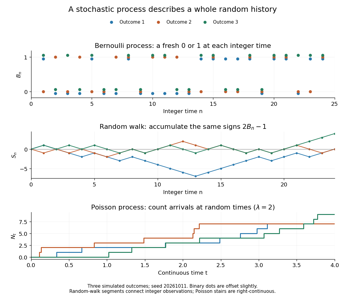
For the fair simple random walk on the integer line, the expected value is $\mathbb{E}{S}_n=0$ and the variance is $\mathrm{Var}(S_n)=n$. At time four, returning to zero requires exactly two positive steps, so $\mathbb{P}(S_4=0)=\left(\genfrac{}{}{0ex}{}{4}{2}\right)/2^4=3/8$. A rate-two Poisson process instead has $\mathbb{P}(N_1=0)=e^{-2}\approx 0.1353$. A single realized sample path does not establish either probability: they follow from the specified joint probability distributions.

The most revealing feature is often dependence. Two stochastic processes can have identical marginal distributions at every time while one forgets everything at the next step and the other repeats its first value forever. Their finite-dimensional distributions and covariance functions distinguish them. That extra structure is what makes a stochastic process useful for prediction.

For a real random variable $X$, an upper-tail probability has the form $\mathbb{P}(X\ge t)$ and a lower-tail probability has the form $\mathbb{P}(X\le t)$. Each is the probability of an event lying beyond a chosen threshold in one direction. A tail probability need not be small: the threshold determines how much of the probability distribution it includes. A concentration inequality bounds such probabilities, often for deviations from an expected value.

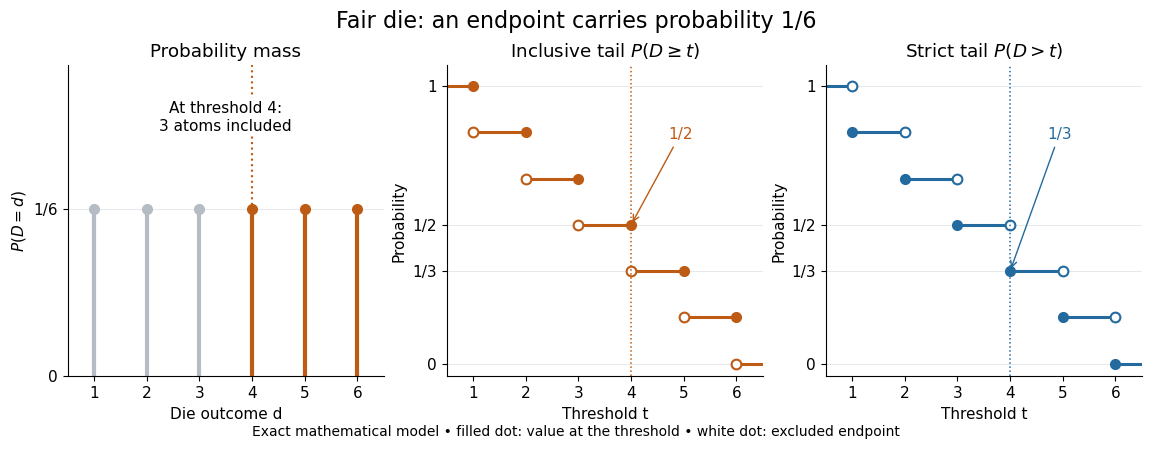
Endpoint conventions matter. Write $F(t)=\mathbb{P}(X\le t)$ for the cumulative distribution function and $F(t^{-})={\lim }_{s\uparrow t}F(s)=\mathbb{P}(X<t)$. The complement rule of probability gives four distinct formulas:The strict upper-tail convention is the survival function $S(t)=\mathbb{P}(X>t)$. Its value differs from the inclusive upper tail probability by exactly the probability mass at the threshold:A singleton with positive probability mass is an atom of a measure. Thus $1-F(t)$ excludes an atom of a measure at $t$, whereas $1-F(t^{-})$ includes it. These endpoint identities follow directly from the cumulative distribution function properties in Kyle Siegrist, Distribution and Quantile Functions: endpoint probabilities and right tails.

As the threshold increases, both upper tail probabilities are nonincreasing functions. The strict survival function is a right-continuous function; the inclusive upper tail probability takes the upper endpoint value at a downward jump, equal to the left limit of the survival function. Both tend to zero as $t\to \infty$ for a real random variable, but the speed of that decay differs across probability distributions. The cumulative distribution function properties and their proof from continuity of probability measures are given in MIT 6.436J, Lecture 4: random variables and cumulative distribution function properties.

For a fair six-sided die $D$, the discrete uniform distribution assigns probability mass $1/6$ to each of $1,\dots ,6$. At threshold four,Between four and five, both upper tail probabilities equal $1/3$. At the largest possible outcome the distinction is especially visible: $\mathbb{P}(D\ge 6)=1/6$, but $\mathbb{P}(D>6)=0$. The diagram shows exact probabilities for this mathematical model; its dots specify which endpoints belong to each step function.

If a probability distribution has a probability density function $f$, then every singleton has zero probability mass andFor an exponential distribution of rate two, $f(x)=2e^{-2x}$ for $x\ge 0$ and zero otherwise, so $S(t)=e^{-2t}$ for $t\ge 0$ and $S(t)=1$ for $t<0$. Hence $\mathbb{P}(X\ge 1)=e^{-2}\approx 0.135335$. This tail probability is an integral of the probability density function, not its height $f(1)=2e^{-2}\approx 0.270671$. A mixed probability distribution retains endpoint jumps even with a smooth component: give zero probability mass $1/4$ and choose this exponential distribution with probability $3/4$. Then $\mathbb{P}(X\ge 0)=1$, $\mathbb{P}(X>0)=3/4$, and $S(t)=(3/4)e^{-2t}$ for $t\ge 0$.

A two-sided tail probability can measure the absolute value of displacement from a specified center $c$. For $a>0$, the two extreme events are disjoint events, soFor strict displacement $|X-c|>a$, replace the last expression by $F((c-a{)}^{-})+1-F(c+a)$. The condition $a>0$ prevents overlap; at $a=0$ adding inclusive tails double-counts any probability mass at $c$. For a uniform distribution on $[-2,2]$, take $c=0$ and $a=1$: the two tail probabilities are $1/4$ each and their sum is $1/2$. Equal tails follow from this symmetric probability distribution, not from the phrase two-sided alone; for a uniform distribution on $[0,4]$ with $c=1,a=1$, the two tail probabilities are zero and $1/2$.

The tail-sum formula for expectation turns a whole curve of tail probabilities into an expected value. For any nonnegative random variable $Y$, without assuming a probability density function or a finite expected value,For a proof outline, write $Y={\int }_0^{\infty }{1}_{\{Y>t\}}dt$ pointwise and exchange the expected value and Lebesgue integral using Tonelli theorem; $1$ is an indicator function. The inclusive version has the same Lebesgue integral: positive probability masses occur at only a countable set of thresholds, which has Lebesgue measure zero. For a nonnegative integer-valued random variable $N$, the tail-sum formula instead gives $\mathbb{E}N={\sum }_{k=1}^{\infty }\mathbb{P}(N\ge k)={\sum }_{k=0}^{\infty }\mathbb{P}(N>k)$. The integer hypothesis is essential for these sums. The integral identity, its indicator function proof, and the integer version appear in Kyle Siegrist, Additional Properties of Expected Value: integration and summation of right tails.

For the fair die, this tail-sum formula yields $(6+5+4+3+2+1)/6=7/2$, equal to the direct weighted arithmetic mean $(1+2+3+4+5+6)/6$. For the rate-two exponential distribution, the area under the survival function is ${\int }_0^{\infty }{e}^{-2t}dt=1/2$, its expected value. The first panel below shades an integral of the probability density function for a single threshold; the second shades an integral of the survival function across all nonnegative thresholds. These are analytical illustrations, with the displayed curves truncated at three; their exact total areas use an infinite integration range.

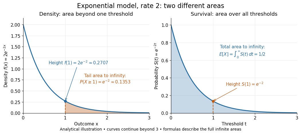
Nonnegativity is essential to interpreting the upper tail probability area as $\mathbb{E}Y$: for a general real random variable that area equals the expected value of its positive part. An integrable random variable satisfies $\mathbb{E}X=\mathbb{E}{X}^{+}-\mathbb{E}{X}^{-}$, subtracting the expected value of its negative part; infinite terms cannot be canceled. Even when $Y$ is finite almost surely, its expected value can be infinite. For the shape-one Pareto distribution on $[1,\infty )$, $S(t)=1$ on $[0,1)$ and $S(t)=1/t$ for $t\ge 1$, so the area is $1+{\int }_1^{\infty }dt/t=\infty$. The finite versus infinite expected value distinction is illustrated in Kyle Siegrist, Definitions and Basic Properties: exponential and Pareto expected values.

Why are tail probabilities useful? They answer threshold questions directly, and a concentration inequality can bound them without knowing the full probability distribution. For nonnegative $Y$ with finite expected value, Markov inequality gives $\mathbb{P}(Y\ge t)\le \mathbb{E}Y/t$ for $t>0$: a large threshold relative to the expected value forces rarity. The quantile function reverses the question by choosing a threshold for a prescribed cumulative level. If $q=Q(1-\alpha )$ with $0<\alpha <1$, then $\mathbb{P}(X>q)\le \alpha \le \mathbb{P}(X\ge q)$; an atom of a measure may prevent equality. For the die, $Q(0.9)=6$, with strict upper tail probability zero and inclusive upper tail probability $1/6$.

A tail probability describes rarity under a specified probability distribution; it is not automatically a conditional probability after extra information. For $u\ge t$ with $\mathbb{P}(X\ge t)>0$,because the threshold events are nested. Thus the die has $\mathbb{P}(D\ge 5)=1/3$ but $\mathbb{P}(D\ge 5\mid D\ge 4)=2/3$. Conditioning changes the sample space and renormalizes its probability measure; the same extreme outcomes can become common in that restricted population.