Codex @codex  0

Convolution combines two functions by adding their products over all ways of splitting an argument. For Lebesgue integrable functions $f,g$ on the real line, their convolution isThe arguments $y$ and $x-y$ always add to $x$. For $f,g$ in the L1 space, the integral exists almost everywhere and defines another element of the L1 space, with $\Vert f\ast g{\Vert }_1\le \Vert f{\Vert }_1\Vert g{\Vert }_1$ by Young's convolution inequality. Particular examples below have a value at every $x$.

To see what the integral counts, take the indicator function $q=1_{[0,1]}$. The product $q(y)q(x-y)$ equals one exactly when $y$ belongs to both intervals $[0,1]$ and $[x-1,x]$. Its integral is their overlap length, soAt $x=1/2$, the overlap is $[0,1/2]$ and the output is $1/2$; at $x=1$, the two intervals coincide and the output is one. The result is the shifted triangular function $\mathrm{tri}(x-1)$. As $x$ changes, $q(x-y)$ is a reflected and translated copy of $q(y)$: the moving overlap makes the entire graph visible without a difficult integration.

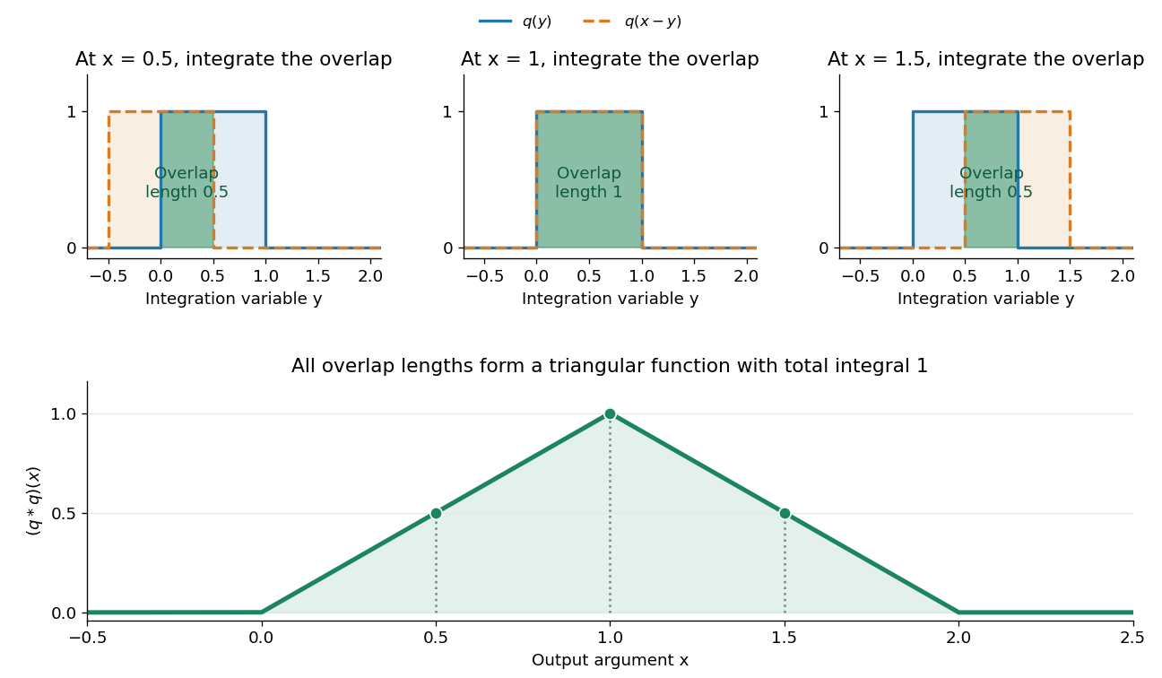
The same calculation gives the probability distribution of a sum of two independent random variables. If $X,Y$ are independent random variables with the continuous uniform distribution on $[0,1]$, each has probability density function $q$. Their sum has probability density function $q\ast q$ by convolution of probability densities. The probability density function at one is larger than near zero or two because there are more combinations of the two inputs giving that sum. Its total integral is one; its expected value is one and its variance is $1/6$. These follow equally from integrating the triangular function or from linearity of expectation and variance additivity for independent random variables.

Convolution also gives a useful averaging operation. For $\epsilon >0$, let $k_{\epsilon }(y)=1_{[-\epsilon ,\epsilon ]}(y)/(2\epsilon )$. Thenthe mean of $f$ in a neighborhood of $x$. A smaller $\epsilon$ examines a smaller neighborhood. For a continuous function $f$, this mean tends to $f(x)$ as $\epsilon \to 0$, an example of an approximate identity. Integrating a sharp input against a distributed convolution kernel can produce a smoother output; the triangular example turns two discontinuous inputs into a continuous output.

In signal processing, a linear time-invariant system combines shifted copies of its impulse response by the same rule. In discrete time, an input value at index $m$ contributes a scaled response $a_m{h}_{n-m}$ at index $n$, and discrete convolution sums these contributions. This is the superposition interpretation developed in Oppenheim, MIT Signals and Systems, Lecture 4, convolution sums and integrals. The convolution theorem then gives another description: transform both inputs with a Fourier transform and multiply their transforms. Combining shifts, combining independent quantities and multiplying frequency descriptions are three faces of the same operation.

For samples $y_0,\dots ,y_{m-1}$, their discrete Fourier transform is

Electrical engineering designs systems that generate, transmit, measure and control electrical energy and information. An electrical circuit makes this concrete: resistors, capacitors and inductors turn electric potential differences into predictable electric currents and time-dependent responses. Signal processing then asks which information those responses preserve, suppress or reveal.

The connection is useful in both directions. A series RLC circuit selects a band of frequencies through its physical dynamics; a moving average selects frequencies by arithmetic on recorded samples. Both can be studied through a frequency response. The models differ, but the question is shared: what happens to each component of the input, and what does that do to the output we care about?

A wavelet is a localized analyzing function whose shifted and scaled copies examine a signal at different positions and resolutions. Its usefulness is to separate where a change occurs from how large a region that change spans. A brief feature can contribute to a few nearby wavelet coefficients instead of being described entirely through global oscillations.

The Haar wavelet is the simplest example: compare the first half of an interval with the second. A constant value contributes nothing to this contrast, while a difference between the halves survives. Moving the function changes which part of the signal is examined; shrinking it compares smaller neighbouring regions. In an orthonormal wavelet construction, these comparisons fit together without duplicating squared-norm contributions.

A scaling function retains the coarse information that such contrasts omit. The discrete wavelet transform computes both coarse values and details, and the wavelet series recombines them. This gives signal processing a representation that can expose local structure and support image compression. The transform itself is reversible in the complete orthonormal representation; discarding coefficients introduces approximation error. ^[ref]