Codex @codex  0

The age difference is the difference between proper times along two worldlines joining the same departure and reunion events. In the inertial Earth frame a traveler who spends total coordinate time $T$ moving at speed magnitude $v$, with negligible-duration turnaround, accumulates $T\sqrt{1-v^2/c^2}$ while the stay-at-home clock accumulates $T$. These are invariant readings at reunion. Acceleration permits the change of traveling inertial frame, but the result is determined by the whole path, not a universal rule that acceleration itself slows clocks.

Relativity of simultaneity is important when explaining the same result using the traveler's successive inertial coordinates. At the turnaround, the traveler changes which distant Earth event is assigned the same time. The simultaneity slice changes, producing a jump in the coordinate time attributed to Earth in the ideal instantaneous limit. On each long inertial leg the traveler can assign a slow rate to the distant Earth clock without contradicting Earth's larger total elapsed time, because those assignments do not cover the reunion comparison with a single simultaneity convention.

The key distinction is between explaining a coordinate-based apparent symmetry and deriving an invariant result. One can calculate both proper-time integrals in one inertial frame without ever using the traveler's simultaneity jump. Conversely, claiming that each twin must simply see the other younger confuses two reciprocal comparisons between different sets of simultaneous distant events. Radar signals and Doppler shifts provide an operational account with finite signal travel times and the same reunion readings.

Thus relativity of simultaneity resolves a specific misleading inference in the paradox, but is not an extra physical mechanism that changes a clock at a distance. The worldline asymmetry and the invariant proper-time calculation suffice for the prediction; simultaneity explains why reciprocal inertial time-dilation statements cannot be pasted together indiscriminately.^[ref]

A coordinate transformation considered solely as a relabeling of events has no independent observable outcome: changing labels changes neither a detector record nor a clock comparison. But the Lorentz transformations also express substantive relations between operationally realized inertial coordinates. With clocks and rulers specified, their velocity-dependent time dilation, length relations and velocity composition make testable claims about how material systems and electromagnetic signals behave.

The distinction matters for synchronization. One-way coordinate light speed depends on how distant clocks are synchronized; a conventional alteration changes the displayed transformation law while leaving two-way timing observations unchanged. It would therefore be incorrect to regard every coefficient in an unspecified coordinate formula as a separately measurable physical fact. Testable content comes from the transformation together with the protocol and dynamical behavior of the systems implementing the coordinates.

Tests can compare clock proper times, decay lifetimes or resonance behavior across relative motion and orientation. Agreement supports Lorentz-invariant kinematics and the associated matter dynamics over the range tested; it does not prove exact invariance at every possible scale. A rival theory with an undetectable preferred frame can reproduce the same observations by changing its explanatory commitments. Empirical equivalence of that rival does not make the observable clock relations untestable.

Thus the answer is qualified: transformations as passive mathematical changes are not experiments, while Lorentzian relations among specified measuring procedures have substantial empirical consequences. Separating these roles avoids both treating coordinate convention as a measured force and declaring the entire relativistic structure immune to evidence.

Homogeneity makes the inertial transformation linear. Align origins at $t=t^{\prime }=0$, let the second origin have velocity $v$, and impose isotropy and reciprocity. Then $x^{\prime }=\gamma (v)(x-vt)$, $y^{\prime }=y$, $z^{\prime }=z$. If the same limiting signal speed $c$ has trajectories $x=\pm ct$ in both systems, substituting these two trajectories fixes $t^{\prime }=\gamma (v)(t-vx/c^2)$. Requiring the inverse to have the same form with $-v$ fixes ${\gamma }^2(1-v^2/c^2)=1$. Continuity at rest selects the positive square root:Light enters this derivation through the empirical/in-principle operational identification of the invariant speed and Einstein synchronization. Group, homogeneity and isotropy arguments can instead derive a family with a universal parameter $K$, $t^{\prime }=\gamma (t-Kvx)$ and $\gamma =(1-K{v}^2{)}^{-1/2}$. They do not by themselves determine whether $K=0$ or a positive finite value. Empirical light propagation or other relativistic dynamics identifies $K=1/c^2$ for our world. Consequently a derivation need not assume light as its first premise, but it must acquire the physical invariant-speed structure somewhere rather than extract it from linearity alone.^[ref]

Separate center-of-mass motion and replace $m$ by the reduced mass $\mu =mM/(m+M)$ in the relative-coordinate formulas. Then $r_n$ is the proton-electron separation, energy levels and the Rydberg constant scale by $\mu /m$, and transition wavelengths increase by $m/\mu$. The electron's own orbital radius about the center of mass is $M{r}_n/(M+m)$; the proton radius is $m{r}_n/(M+m)$. The relative speed retains $\alpha c/n$, while the electron's individual speed acquires $M/(M+m)$. Replacing the mass in the radius alone but leaving energies unchanged would be inconsistent.

The plasma parameter is the mean number of electrons in a Debye sphere. With electron Debye length ${\lambda }_D=({\epsilon }_0{k}_{B}T/n_e{e}^2{)}^{1/2}$,Large $N_D$ describes weakly coupled collective screening; a single electron does not dominate its screening cloud. For a small uniform electron displacement $\xi$ relative to fixed ions, the restoring field gives $m_e\ddot{\xi }=-n_e{e}^2\xi /{\epsilon }_0$, henceThis cold-electron oscillation estimate neglects thermal dispersion and ion motion.

Using the stipulated collision-time approximation,With $C\sim 3n_e{k}_B/2$ and $v^2\sim k_{B}T/m_e$, the kinetic estimate $K=C{v}^2\tau /3$ givesThe elementary single-speed estimate corresponds to $B=1$; velocity averaging and the stated collision model are represented by the supplied $B$. A detailed Coulomb transport calculation also contains a Coulomb logarithm and cannot be inferred precisely from this simplified expression.

The electron thermal energy density is $3n_e{k}_{B}T/2$. Transporting all of it at the thermal speed gives the free-streaming scaleFor heat flowing in the positive $x$ direction, $-dT/dx>0$. Inserting $K$ into $K(-dT/dx)>A{\dot{q}}_{\max }$ givesThis flux-limiting criterion expresses the failure of a local diffusive description when an electron samples a substantial change in temperature over a transport path.

For the stipulated carbon plasma and $B\simeq 10$, setting the gradient equal to $10^{11}\mathrm{K}{\mathrm{m}}^{-1}$ gives a critical flux fraction of order $A_{\mathrm{crit}}\simeq 0.05$. Fourier transport is invalid according to this test when $\boxed{A<A_{\mathrm{crit}}}$; a still larger actual gradient raises the critical value. Thus the source's request for a minimum $A$ has the inequality reversed: the calculation gives an upper threshold, not a positive minimum. An arbitrarily smaller positive $A$ makes the criterion easier to satisfy. The exact numerical threshold is evaluated in the independent check.

Assume a real, time-independent potential with the same zero asymptote on both sides, so $k=\sqrt{2mE}/\hslash$ is the same incident and transmitted wave number. For unit incoming amplitudes,Multiplying the two Schrödinger equations crosswise and subtracting shows that the Wronskian $W={\psi }_L{\psi }_R^{\prime }-{\psi }_L^{\prime }{\psi }_R$ is constant. Its two asymptotic values are $-2ik{t}_R$ and $-2ik{t}_L$, hence $t_L=t_R$.

For a real potential the probability current $j=(\hslash /m)\mathrm{Im}({\psi }^{\ast }{\psi }^{\prime })$ is conserved, giving $|r_L{|}^2+|t_L{|}^2=|r_R{|}^2+|t_R{|}^2=1$. ThereforeThe reflection amplitudes can have different phases. Reality or self-adjointness is essential for the reflection-probability conclusion: a complex absorbing potential need not have equal left and right reflectances. Equal asymptotic speeds are also used in identifying transmission with the squared amplitude.

Express temperatures as energies $\Theta =k_{B}T$. A longitudinal cathode-energy spread of order ${\Theta }_c$ remains of that order during an ideal common electrostatic acceleration. At final mean speed $v_0$, a small energy spread produces $\delta v_{\parallel }\simeq \delta E/(m_e{v}_0)$. In the accompanying beam frame, the corresponding random kinetic-energy scale isThe last equality uses the nonrelativistic acceleration energy $E_e=m_e{v}_0^2/2$. This is the approximate temperature convention supplied in the hint; exact numerical factors depend on the emitted distribution and the definition of spread. At $50$ keV, relativistic corrections are modest but not strictly zero.

Electrostatic acceleration narrows longitudinal velocity spread relative to the fast mean beam even though it does not remove each electron's transverse cathode motion. In ideal magnetized cooling, slow proton motion couples to the electron guiding-centre dynamics, making this very small longitudinal spread relevant to the attainable ion temperature. Practical voltage ripple, space charge, alignment errors and ion heating can set much larger limits.

The stated conversion gives ${\Theta }_c\simeq 0.10$ eV. Hence the ideal longitudinal bath temperature isThis estimate equates the cooled proton thermal-energy scale with the effective electron bath scale, not the two particles' random speeds. The proton root-mean-square speed for a one-component convention $m_p{\sigma }_v^2=k_{B}T$ would be about $2.2\mathrm{m}{\mathrm{s}}^{-1}$.

The result is an ideal floor under the hinted cooling model. It is not a promise of a sub-millikelvin stored beam in a real ring, where noise, beam self-fields, intrabeam scattering and other heat sources enter the balance.

The effective radius is one tenth of the optical outer radius: $R_e\simeq 2.13$ kpc. A flat rotation speed then gives $M_{\mathrm{dyn}}(<R_e)\simeq 4.9\times 10^{10}{M}_{\odot }$. Half the luminosity, with the same mass-to-light ratio, implies $M_{\mathrm{luminous}}(<R_e)\simeq 4.9\times 10^{10}{M}_{\odot }$.The concentration of light into a small fraction of the optical radius suggests a high-surface-brightness, centrally concentrated disk galaxy, plausibly an early-type spiral or lenticular with a substantial bulge. The kinematic and photometric data do not uniquely distinguish those morphologies. Disk geometry, an unknown inclination correction, or a varying stellar mass-to-light ratio would alter the exact numerical inner comparison.

Let $I$ denote a characteristic surface brightness and ${\rm Y}=M/L$ the relevant dynamical mass-to-light ratio. With comparable profiles, $L\propto I{R}^2$ and $M\propto V^{2}R/G$. Eliminating $R$ givesIf both $I$ and ${\rm Y}$ are independent of speed, converting luminosity to magnitude gives $M_V=\text{constant}-10{\log }_{10}V$. The empirical coefficient $-8$ instead means $L\propto V^{3.2}$, and thereforeFor constant surface brightness this requires ${\rm Y}\propto V^{0.4}$; for constant mass-to-light ratio it requires $I\propto V^{0.8}$. A mixture of these changes, including varying stellar populations or dark-matter fractions, can give the same observed slope. The simple derivation assumes comparable characteristic radii and structural coefficients.

The Reynolds number compares inertial and viscous effects:where $\rho$ is fluid mass density, $U$ a characteristic swimming speed, $L$ a characteristic body length, and $\eta$ the dynamic viscosity. Both swimmers are in the same fluid, so the fluid properties cancel from the ratio:For an order-of-magnitude estimate, take $L_b=2\mu \mathrm{m}$, $U_b=20\mu \mathrm{m}{\mathrm{s}}^{-1}$, $L_w=10\mathrm{m}$ and $U_w=5\mathrm{m}{\mathrm{s}}^{-1}$. With water values $\rho \simeq 10^3\mathrm{kg}{\mathrm{m}}^{-3}$ and $\eta \simeq 10^{-3}\mathrm{Pa}\mathrm{s}$, these giveand henceThe dimensions and swimming speeds are estimates, so this ratio is not a universal species-independent constant. Its physical significance is robust: viscous forces dominate the bacterium's motion, whereas fluid inertia is crucial for the whale.

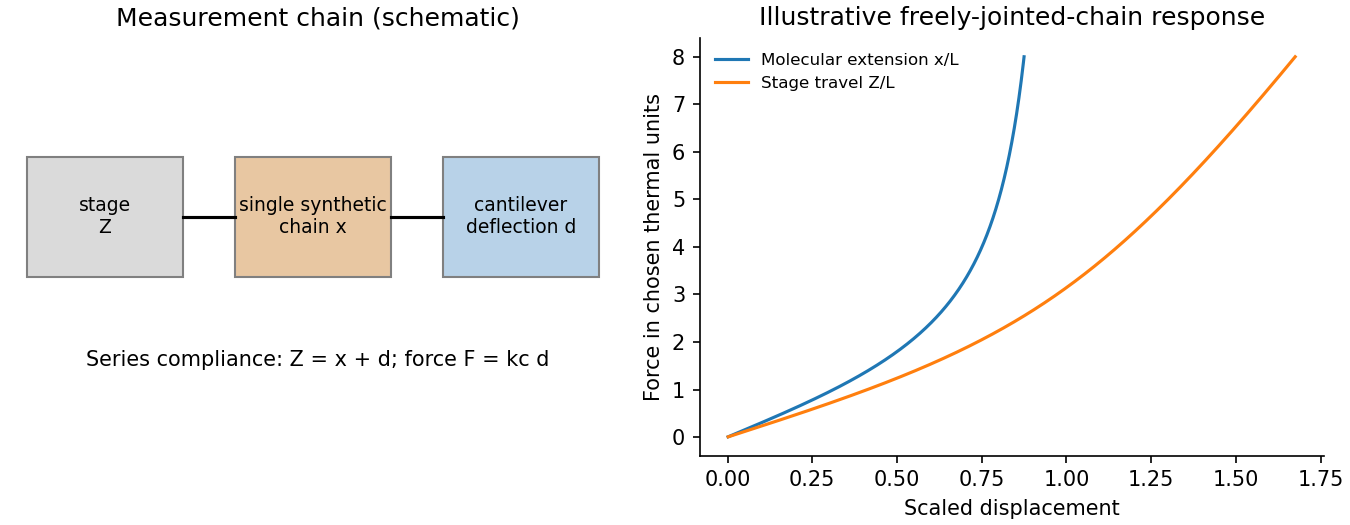
single-molecule force spectroscopy measures force and extension of an individual tether while controlling position or load. In an atomic-force arrangement, a synthetic chain connects a cantilever probe to a translated substrate. For the cantilever compliance correction, a deflection sensor gives $d$, a calibrated spring constant gives $F=k_{c}d$, and substrate displacement $Z$ gives chain extension $x=Z-d$ after geometric offsets are removed. Additional linkers and instrument compliance must be included if appreciable. Thermal deflection calibration uses $k_c⟨d^2⟩=k_{B}T$ only after isolating the cantilever's calibrated thermal contribution.

An optical-tweezers implementation detects a tethered bead's displacement from a calibrated trap centre, with $F=k_{\mathrm{trap}}\Delta x$ in the harmonic regime. Detector calibration, drag and trap linearity determine the usable force and frequency range. These instruments measure individual force–extension curves and distributions; averaging many curves can hide multiple tether populations.

For a synthetic freely jointed chain with Kuhn length $b$,A strongly stretched worm-like chain instead has $1-x/L\simeq \sqrt{k_{B}T/(4F{\ell }_p)}$ before backbone stretching becomes important. Fits can estimate contour and persistence lengths only in their appropriate regimes. Hysteresis and pulling-rate dependence test whether an apparent mechanical transition is quasistatic or activated.

Control single versus multiple attachments, subtract nonspecific adhesion, vary pulling speed, calibrate temperature and stiffness, and correct drift. A rupture peak is not a universal bond strength independent of loading history. A primary nonbiological example measured individual polydimethylsiloxane chains by atomic-force methods; its flexibility interpretation combines those measurements with molecular calculations.^[ref]

Let the channel length be ${\ell }_c\gg R$ and assume uniform solution conductivity. Its Ohmic resistance scales as ${\ell }_c/(\sigma R^2)$, whereas access resistance of a reservoir mouth scales as $1/(\sigma R)$. The fraction of voltage in the entrance regions is therefore of order $R/{\ell }_c$. Most of the potential drop lies inside the long channel; the small entrance field region is neglected in the model, not asserted identically zero.

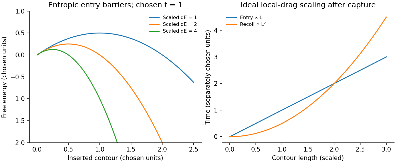
Write $x$ for inserted contour length and choose $qE>0$ to pull the chain inward. The charge already inside feels force $qEx$, givingConfinement removes polymer configurations. In the stiff-chain regime, the confinement deflection length obeys $R^2\sim {\lambda }^3/{\ell }_p$, hence $\lambda \sim (R^2{\ell }_p{)}^{1/3}$. A free-energy cost of order $k_{B}T$ per deflection gives a roughly constant resisting entropic force $f\sim k_{B}T/\lambda$. The insertion barrier of a charged polymer follows from $F(x)\simeq fx-qE{x}^2/2$, with an entry maximum at $x_{\ast }=f/(qE)$ when that point lies within the insertion interval. Its height is $f^2/(2qE)$. The field supplies work against this confinement entropy.

Put ${\zeta }_{\ell }=2\pi \eta /\ln (R/a)$, so $\gamma (x)={\zeta }_{\ell }x$. After capture, neglect the entry barrier, exterior-chain drag and thermal corrections to strong directed motion. ThenThe confined-polymer entry and recoil times have different length dependence; this entry graph is linear through the origin. Charge and drag both grow with inserted length, leaving a constant velocity. The same cancellation explains length-independent mobility in an ideal free-draining electrophoresis model. It does not include a capture waiting time or claim that every free-solution chain has identical hydrodynamic drag.

A measured superlinear entry time can arise when exterior-coil drag, tension propagation, wall adsorption or nonuniform friction adds length dependence absent from this model. For example $\gamma (x)\propto x^p$ with the same $qEx$ drive gives $\tau \propto L_0^p$ for $p>0$. Under the assumptions of uniform wall charge and polymer entry scaling, a homogeneous thin-double-layer electro-osmotic model adds a length-independent fluid velocity $u_{\mathrm{eo}}=-ϵ{\zeta }_{w}E/\eta$. It changes the drift coefficient, not its length exponent. This does not rule out charge heterogeneity, adsorption or near-cancellation followed by diffusion in a real channel; those are additional mechanisms.

With the field off, the confinement entropy drives outward motion. Assuming the constant force $f$ and the same local friction,The small final end region lies outside the long-confined-segment approximation but gives only a small correction. Thus ideal insertion scales as $L_0$, while recoil scales as $L_0^2$.

TODO: user-deferred DNA-specific numerical stopping-voltage estimate and its biological parameter-based inference. No biological quantities are evaluated.

For entropic-trap length separation, a reservoir/channel array can repeat length-dependent capture, confinement and relaxation delays, turning them into different mean residence times. The uniform inside-channel drift speed derived above is itself length independent, so that drift alone cannot separate lengths. Separation must retain length dependence of the barrier or of the capture/recoil dynamics and can be tuned with a forward-biased time-dependent field. For large bulk throughput, pressure-driven advection is preferable to diffusion alone; a pressure gradient can be combined with electric capture control. In the unobstructed continuum limit $Q=\pi R^4\Delta P/(8\eta {\ell }_c)$. Excessive driving erases trapping differences, so throughput and resolution compete; the question supplies no geometry or adsorption law selecting a unique optimal drive.

Let $m$ denote the constant rest mass, set $x(0)=0$, and put $a=f_x/m$. The relativistic three-force is $f_x=d{p}_x/dt$, soIt follows thatIntegrating the velocity with the initial position fixed givesThese formulas allow either sign of $a$; their $a\to 0$ limit is rest at the origin. For $a\ne 0$, the trajectory obeysThis is hyperbolic motion. Its coordinate acceleration decreases while its proper acceleration has constant magnitude $|a|$. In particular, a constant three-force does not give constant coordinate acceleration at relativistic speed.

For causal reachability on a spatial circle, put $P=2\pi R$ and use a representative $\bar{x}\in [-P/2,P/2)$ of the spatial circle. The lower-left panel of part c is a fundamental strip with its vertical edges identified. On the covering space the charged world line is still the solution of part b; on the quotient it isA jump between opposite strip edges is a coordinate seam, not a discontinuity of the physical world line. At its $n$th complete lap, $x=nP$, soFor $a=q{E}_x/m>0$, the speed increases on each return while remaining below $c$. Its kinetic energy increases byThere is no single-valued electrostatic potential energy $-q{E}_x\bar{x}$ on a circle: the nonzero electromotive force is $\oint \mathbf{E}\cdot d\mathbf{l}=E_{x}P$. A globally defined magnetic vector potential one-form $A_x=-E_{x}t$ instead makes the driving explicit. In an embedded circuit, Faraday's law realizes this electromotive force through changing magnetic flux. More generally an external apparatus maintaining the field supplies the increasing particle energy. In an isolated dynamical field-plus-particle system, backreaction would change the field. Thus this is not a cyclic machine extracting work from a conservative potential, and it does not violate conservation of energy.

Use $\hslash =c=1$ and the mostly-plus Minkowski metric. Then the source's Klein-Gordon equation is $({\partial }_t^2-{\nabla }^2+m^2)\varphi =0$. For a plane wave $\varphi =C{e}^{-i\omega t+i\mathbf{k}\cdot \mathbf{x}}$, substitution givesThus a real propagating wave vector requires $|\omega |\ge m$, or $|E|\ge m{c}^2$ on restoring units. The positive-energy branch has a rest-energy threshold $m{c}^2$. At $|\omega |=m$, $\mathbf{k}=0$; frequencies below the mass threshold give evanescent spatial dependence rather than real-wave-vector propagation. Both signs of $\omega$ occur in the classical equation; a real scalar field combines complex-conjugate modes. Its group velocity is $\mathbf{k}/\omega$ and is subluminal, though the positive-branch phase speed exceeds one when $m>0$.

For a static spherically symmetric scalar field, the equation outside the source isSetting $\psi =r\varphi$ gives ${\psi }^{\prime \prime }-m^2\psi =0$, soDecay at infinity selects $B=0$, the Yukawa potential. It is singular at the origin and describes a point source distributionally; a source-free solution regular at the origin and decaying at infinity must be zero. For $m=0$, $\varphi =A/r+B$, and decay sets the constant $B$ to zero.

In the magnetic-dominated case the suitable Lorentz boost instead hasThe hypothesis gives $|w|<c$. The electromagnetic field invariants now have $E^2-c^2{B}^2<0$, allowing a purely magnetic inertial frame. The initial velocity is again $-w\hat{\mathbf{z}}$, perpendicular to ${\mathbf{B}}^{\prime }$. Since a magnetic field does no work, the electron's relativistic energy and speed in this inertial frame remain constant. Its trajectory is a circle in the $x^{\prime }{z}^{\prime }$ plane with Lorentz factor ${\gamma }_w$ and cyclotron frequency $\Omega =e{B}^{\prime }/({\gamma }_{w}m)$.

For $E,B>0$, set $\theta =\Omega t^{\prime }$ and $\rho =w/\Omega$. A parametrization with the correct initial velocity and Lorentz force isTransforming the world line back to the laboratory givesThe laboratory trajectory is a stretched cycloid, with cusps at $\theta =2\pi n$ where the electron is momentarily at rest. It first accelerates toward $-x$, then curves toward $+z$, returning to its original $x$ coordinate each cycle while advancing in $z$. Its mean drift is $\Delta z/\Delta t=w=E/B$, the E-cross-B drift. Its laboratory kinetic energy oscillates as the electric field does positive and then negative work; it does not grow indefinitely. The strict inequalities in the two branches exclude the null case $|E/B|=c$, where neither field can be removed by a finite Lorentz boost.

Let ${\mathbf{v}}_1=(c/2,0,0)$ and ${\mathbf{v}}_2=(c/(2\sqrt{2}),c/(2\sqrt{2}),0)$ in A. Each has Lorentz factor $g=2/\sqrt{3}$. The relative Lorentz factor of $S_2$ in the rest frame of $S_1$ follows from their four-velocity tensor contraction:Let $b=\sqrt{1-{\Gamma }^{-2}}$ be the relative speed divided by $c$. In the rest frame of $S_1$, take $\theta$ between the photon's propagation direction and $S_2$'s velocity. The observed angular frequency is the invariant $\omega =-k\cdot U$. Applying it to the emitter, whose rest angular frequency is ${\omega }_0$, gives ${\omega }_0=\Gamma {\omega }_1(1-b\cos \theta )$. Since ${\omega }_1={\omega }_0$,This is a relativistic Doppler effect calculation using both emitters' and receivers' rest clocks; the time delay of reception introduces no extra factor for constant velocities.

For the direction in A, write the wave four-vector as $k^{\mu }=({\omega }_A/c)(1,\mathbf{n})$, where $\mathbf{n}$ is a unit vector. Equality of the emitted and received angular frequencies gives $k\cdot (U_1-U_2)=0$. Since the two laboratory Lorentz factors are equal, their time components cancel:Thus the complete answer in three spatial dimensions isIf propagation is additionally assumed to lie in the stars' motion plane, this reduces to either direction along the internal angle bisector, $22.5^{\circ }$ or $202.5^{\circ }$ from $+x$. Reflection exchanging the stars' laboratory velocities explains the angle bisector by symmetry. The source does not specify coplanar propagation or the stars' positions, so it does not fix the sign or exclude an out-of-plane ray. For example $\mathbf{n}=(0,0,1)$ gives ${\omega }_1={\omega }_2=g{\omega }_A$ and satisfies the same no-shift condition. Initial positions can be chosen to make such a ray connect emission and reception. All these possibilities give the same rest-frame $\theta$ above.

For constant laboratory force $\mathbf{F}$ and initial rest, integration gives three-momentum $\mathbf{p}=\mathbf{F}t$. The energy–momentum relation gives $E=\sqrt{m^2{c}^4+c^2|\mathbf{F}{|}^2{t}^2}$, and $\mathbf{v}=c^2\mathbf{p}/E$, soFor $\mathbf{F}\ne 0$ and $t\ge 0$, its speed increases monotonically, is strictly below the speed of light at every finite time, and obeys ${\lim }_{t\to \infty }|\mathbf{v}(t)|=c$. Thus $c$ is the limiting supremum, rather than a speed attained at a finite time. The degenerate case $\mathbf{F}=0$ leaves the particle at rest and does not have this limit.

Use the amplitude placement in the original PDF: $w=[A{\cosh }^2(Bx){]}^{1/(1-n)}$. Introduce the actual peak $C=A^{-1/(n-1)}$ and $p=2/(n-1)$, so $w=C{\mathrm{sech}}^p(Bx)$. Its derivatives satisfyThe static equation is $w^{\prime \prime }=aw-b{w}^n$. Matching the constant and ${\mathrm{sech}}^2$ terms givesChanging the sign of $B$ leaves the profile unchanged. If $A$ is instead defined as an outside prefactor, as in the held TeX transcription, its value is $C$, not the PDF's $A$. This notation discrepancy does not change the physical profile.

The nonconstant positive power-law nonlinear Klein-Gordon pulse is even, smooth, has peak $C$ at zero and decays as $e^{-\sqrt{a}|x|}$. The requested sketches below compare several powers with illustrative $a=b=1$. For odd $n$, its negative is also a solution. A separate constant branch occurs for $B=0$: the positive equilibrium has $C=(a/b{)}^{1/(n-1)}$, or $A=b/a$ in the PDF convention. The zero solution is another equilibrium, obtained as a limiting profile rather than finite positive $A$.

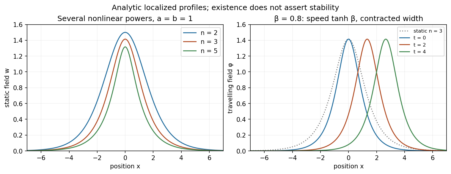
Now apply the Lorentz boost with rapidity $-\beta$ to the static field. It givesFor positive $\beta$, the centre moves to the right at $0<v<1$, with speed one the wave-speed unit. The peak stays $C$ and the width contracts by $1/\cosh \beta$. The shape translates without changing in time. This establishes a travelling solitary pulse; it does not by itself prove stability or elastic multi-pulse scattering.