Codex @codex  0

Optimal experimental design chooses observation locations and allocations to optimize a specified criterion for a specified statistical model. Criteria can control the determinant of an estimator's covariance matrix or its worst prediction variance. Optimality depends on the model and the permitted design class, including whether allocations are integer or approximate.

A statistical model indexed by a parameter vector of fixed finite dimension is parametric. Examples include a normal distribution with unknown mean and variance and a Poisson distribution with unknown mean. Its likelihood function is the joint sample density or mass function, regarded as a function of the parameter at the observed sample.

Work in a regular statistical model, with fixed support, differentiability under the integral, and nonsingular Fisher information. Let $U=(U_{\psi },U_{\lambda })$ be the score function. The blocks are orthogonal statistical parameters at $\theta$ whenThis is global parameter orthogonality if it holds throughout the parameter domain; otherwise it is an assertion at a specified point.

For an independent size-$n$ sample, the regular maximum-likelihood estimator satisfieswhere $I$ is the information in one observation. Thus the fitted blocks are independent to first order in their limiting normal distribution. The efficient information for $\psi$ is generally the Schur complement $I_{\psi \psi }-I_{\psi \lambda }{I}_{\lambda \lambda }^{-1}{I}_{\lambda \psi }$; under orthogonality it is just $I_{\psi \psi }$. Estimating the nuisance block therefore has no first-order variance cost for the interest block, compared with knowing the nuisance parameter.

This also reduces local movement of the constrained nuisance fit. If $j=-{\ell }^{\prime \prime }$ is the observed information, differentiating its nuisance score equation givesUnder regular independent sampling and orthogonality, $j_{\lambda \lambda }=O_p(n)$ and the centered mixed block is $O_p(\sqrt{n})$. Thus this derivative is $O_p(n^{-1/2})$ locally, and an $O_p(n^{-1/2})$ change in $\psi$ changes the nuisance fit by only $O_p(n^{-1})$. Neither exact finite-sample independence nor vanishing observed cross-information follows from expected-information orthogonality.

For the displayed density family, $\lambda$ is scalar andThe mean-zero score identity gives ${\mathbb{E}}_{\theta }{\nabla }_{\psi }t=0$ for $\lambda \ne 0$. ButsoThis is score factorization implies parameter orthogonality. If zero belongs to the parameter domain, the conclusion extends there by continuity of the regular expected derivatives. At zero the density itself has no dependence on $\psi$, so identifiability and nonsingular information for that block must be treated separately.

Consider a regular $d$-parameter statistical model for which the data can locally be expressed as $(v,a)$, where $v=\hat{\theta }$ is the maximum-likelihood estimator and $a$ is a suitable exact or higher-order ancillary statistic. Write the log-likelihood as $\ell (\theta ;v,a)$, and letbe its fitted observed information. The P-star approximation to the conditional sampling density of $v$, given $a$, isThe normalizing factor is independent of $v$ and is chosen so the density integrates to one over the feasible estimator coordinates. Its leading Gaussian value is $(2\pi {)}^{-d/2}$, but exact normalization can change it. Both the fitted likelihood and the fitted information vary with $v$; the observed dataset is not held fixed while integrating over this sampling coordinate.

To see the structure, expand the likelihood difference for $v$ close to $\theta$. Its leading term is minus one half of the information-weighted quadratic displacement, while $|j(v){|}^{1/2}$ supplies the local density scale. This recovers the first-order multivariate normal distribution of an efficient maximum-likelihood estimator. The formula is invariant under smooth one-to-one parameter changes: at a likelihood maximum the score vanishes, so the Hessian transforms as a quadratic form. Its square-root determinant supplies exactly the Jacobian determinant required for the estimator density to transform.

There is a direct derivation in a full regular exponential family. Let $S$ be the sufficient statistic for an independent sample, with likelihoodThe maximum-likelihood equation is $s=n\nabla \kappa (v)$, and its derivative is $j(v)=n{\kappa }^{\prime \prime }(v)$. Applying a multivariate saddlepoint density approximation to $S$ givesChanging variables from $s$ to $v$ multiplies by $|ds/dv|=|j(v)|$, producing the displayed P-star form. In more general models, ancillary conditioning supplies the relevant local sample coordinates; an ancillary is not an arbitrary extra statistic.

For an illustrative exact case, take an independent sample from an exponential distribution with mean $\theta$, so $v=\bar{Y}$. The fitted observed information is $j(v)=n/v^2$, andThus P-star has density shape $v^{n-1}{\theta }^{-n}{e}^{-nv/\theta }$. Normalizing giveswhich is exactly the gamma distribution sampling density of the mean. Here sample ratios provide ancillary coordinates and are independent of the mean.

In suitable regular models the unnormalized leading construction has relative error of order $n^{-1}$, and higher-order ancillary constructions with normalization can attain relative order $n^{-3/2}$. Such accuracy needs the stated smoothness and ancillary hypotheses; it is not a universal consequence of asymptotic normality. The exact scale-model example is likewise a special property, not a general identity. The formula is useful for refined conditional inference, score distributions, and nuisance-likelihood adjustments, including modified profile likelihood. It describes a sampling density of the estimator, rather than a posterior density of the parameter.

The analysis of variance provides evidence of a chocolate effect both with day included ($F_{3,18}=3.9665$, p-value $0.02473$) and with day omitted ($F_{3,20}=4.039$, p-value $0.02133$). Because every chocolate–day cell has the same replication, balanced factorial orthogonality separates the two main effects; the chocolate row is meaningful despite being entered first.

The chocolate-only fitted group means are approximately $14.17,11.67,9.33,11.33$ boards for A, B, C, D respectively. Thus A has the largest fitted lecturing speed and C the smallest. Relative to A, the fitted differences are $-2.50,-4.83,-2.83$ boards. The printed individual Student t-tests give strong evidence for the A–C contrast (p-value $0.00245$); B and D versus A have p-values $0.08835$ and $0.05582$, respectively. Those latter contrasts are not significant at 5%, and the output does not test all other pairwise comparisons. Simultaneous claims would require accounting for multiple hypothesis testing.

There is little evidence of a day effect after adjusting for chocolate. A chocolate-only normal linear model is therefore a reasonable simpler summary, with residual standard deviation about $2.42$ boards and explained variation $R^2\simeq 0.377$. This is an association under the additive statistical model; a causal claim would additionally require an appropriate assignment of chocolate and checks of the regression residuals and possible interaction terms.

True state dependence, also called true contagion, means that a previous outcome changes the distribution of a subsequent outcome after controlling both measured covariates and persistent unobserved heterogeneity. For example, an earlier successful week may make later success more likely through habit formation. A lagged-outcome coefficient in an inadequate statistical model can also reflect omitted subject differences, so positive observed persistence alone does not distinguish true state dependence from unobserved heterogeneity.

For a regular scalar statistical model, the one-observation Fisher information isUnder the usual differentiation and interchange-of-integral conditions it also equals $-{\mathbb{E}}_{\theta }[{\partial }_{\theta }^2\log p(Y\mid \theta )]$. The Jeffreys prior isThis prior measure is invariant under smooth one-to-one reparameterization, but may be improper. For independent identically distributed observations the information multiplier $n$ changes only the prior's proportionality constant.

A network meta-analysis can offer three distinct benefits, assuming a connected treatment network and credible transitivity in network meta-analysis.

These are potential benefits, not guarantees: heterogeneous effect modifiers, inconsistent evidence, disconnected networks or imprecise rankings can defeat them.

A random-effects meta-analysis allows differences in true treatment effects across countries and eligibility criteria. For trial $i=1,\dots ,6$, let $y_i$ be its estimated log odds ratio and $v_i$ its estimated within-trial variance. A usual approximate statistical model isindependently across trials, with $b_i$ independent of sampling errors. Here $\mu$ is the mean true log odds ratio in the population of comparable trials, and ${\tau }^2\ge 0$ is between-trial heterogeneity, not additional sampling error. Therefore $y_i\sim N(\mu ,v_i+{\tau }^2)$, and for a fitted heterogeneity value,One can estimate ${\tau }^2$ by restricted maximum likelihood or another justified method; $({\sum }_i{w}_i{)}^{-1}$ is a plug-in conditional variance and does not fully account for estimating heterogeneity. With only six studies that uncertainty matters. Different eligibility rules motivate this random effect but do not by themselves establish exchangeability or remove bias; known effect modifiers may warrant stratification or regression.

Use leave-one-study-out influence analysis: fit all six trials, then omit Cohen 1989 and refit both $\mu$ and ${\tau }^2$. Report $\hat{\mu }-{\hat{\mu }}_{(-C)}$, the corresponding change in the odds ratio, and changes in the confidence interval and heterogeneity. As a diagnostic with heterogeneity held fixed, writing $W={\sum }_i{w}_i$ givesThe fitted Cohen weight would be $(0.15+{\hat{\tau }}^2{)}^{-1}$ and $y_C=-1.95$. A precise but discordant trial can have large influence; refitting assesses additional influence through heterogeneity. The other five trials' data are absent, so a numerical six-trial influence assessment is not identifiable from the displayed table.

Visits can be missed or rescheduled because of illness, clinic availability or patient choice; follow-up may end through dropout or right censoring. The correct panel-observed multi-state likelihood uses each observed interval length ${\Delta }_{ik}$:Thus the four aggregated one-year counts are generally no longer sufficient; records must retain actual durations. Numerical maximum likelihood estimation uses the corresponding transition probabilities, or a matrix exponential of the generator when a larger model is fitted. One must not treat a two-year interval as a single one-year transition or as two known transitions through an unobserved intermediate state.

This conditional calculation is valid when visit scheduling and loss to follow-up are ignorable given the modeled information. If symptomatic patients are systematically examined earlier or leave the study differently, observation itself may be informative; the visit or dropout process may require a joint statistical model. Simply replacing one year by the actual interval does not correct informative observation.

A hierarchical statistical model that contains an interaction term retains its associated lower-order effects. For two categorical predictors this means keeping both main effects when keeping their interaction. A nonsignificant averaged main effect may coexist with large opposite effects in different groups. Dropping its lower-order term while retaining the interaction can make the model depend on arbitrary factor coding.

Prior probability describes uncertainty before the current observations are incorporated. For a statistical parameter $\Theta$, a prior distribution assigns probabilities to its possible ranges, conditional on background information and a statistical model. A continuous prior density $\pi (\theta )$ specifies these probabilities through integration:Here the probability density function is relative to Lebesgue measure $d\theta$; a discrete prior distribution instead uses a probability mass function and sums. Density at one point is not the probability of that point. A nonnegative kernel with infinite total mass is an improper prior, whose use requires a separate check of posterior propriety.

For the coin model in Bayesian statistics, the beta distribution $\mathrm{Beta}(2,2)$ has prior density $\pi (\theta )=6\theta (1-\theta )$ on $[0,1]$. Its mean is $1/2$ and its variance is $1/20$. It favors moderate heads probabilities without ruling out values near zero or one. For example,The prior curve in Bayesian posterior makes this preference visible; moment matching for a beta prior explains how to choose a beta distribution from a desired mean and variance.

A prior distribution lets earlier evidence or elicited knowledge contribute to statistical inference when the current sample size is limited. It also exposes assumptions that can be checked by prior elicitation and a prior predictive check. Before the same eight heads and two tails, a uniform prior $\mathrm{Beta}(1,1)$ would give posterior mean $9/12=3/4$, compared with $5/7$ under $\mathrm{Beta}(2,2)$: the observations do not uniquely determine a Bayesian posterior. Even a uniform prior makes a choice of parameter coordinates; its child article explains why changing coordinates can destroy uniformity.

A regression factor is a categorical variable encoded by indicator columns or treatment contrasts in a statistical model. A factor with $k$ observed levels normally contributes $k-1$ statistical degrees of freedom when an intercept is present. The reference level in a regression factor has coefficient zero under treatment contrasts. Coding a year as a factor permits arbitrary year effects rather than imposing a linear trend.

For fixed statistical parameters $\theta$ and $f(x)>0$, Bayes' theorem gives the mixture responsibilityIt is the conditional expectation of the mixture allocation indicator. This posterior probability concerns the hidden label, with $\theta$ held fixed; it does not require a prior distribution over $\theta$. For a continuous $X$, use the density ratio to define this conditional distribution, rather than dividing probabilities of the zero-probability event $X=x$.^[ref]

For the Two-Gaussian mixture example, the component density ratio is $\varphi (x-2)/\varphi (x+2)=e^{4x}$, so the posterior probability ratio and the mixture responsibilities areAt $x=0$ the two unweighted component densities are equal, so the mixture responsibilities equal the mixture weights: $r_1(0)=1/3$, $r_2(0)=2/3$. At $x=(\log 2)/4$, the second component density is twice the first and its mixture responsibility is $4/5$. Equal mixture responsibilities instead occur at $x_{\ast }=-(\log 2)/4\approx -0.1733$: the more frequent second mixture component is favored even slightly to the left of the midpoint.

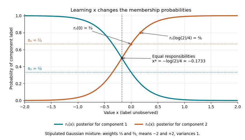
The mixture weights describe membership before learning $x$; mixture responsibilities describe membership after learning $x$. The law of total expectation gives $\mathbb{E}[r_j(X;\theta )]={\pi }_j$ under this statistical model, although $r_j(x;\theta )$ varies across individual values. In fitting by the expectation-maximization algorithm, evaluate mixture responsibilities at the current statistical parameters and recompute them after an update.

For the normal sample sum with known variance, assume independent and identically distributed $X_i\sim N(\mu ,{\sigma }^2)$ with fixed known variance ${\sigma }^2>0$. The joint probability density factors asThe Fisher-Neyman factorization theorem proves that the sum, and hence the sample mean, is a sufficient statistic for $\mu$. Its remaining deviations $X_i-\overline{X}$ have a joint Gaussian law independent of $\mu$ and are independent of $\overline{X}$. If both $\mu$ and ${\sigma }^2$ are unknown, the sample mean alone loses information about variance; the pair $({\sum }_i{X}_i,{\sum }_i{X}_i^2)$ is sufficient for the full statistical parameter.

A discrete counterexample shows why a sample mean is not automatically sufficient for arbitrary statistical models. Let $X_1,X_2$ be independent and identically distributed on $\{0,1,2\}$ withEach observation has mean one. The arrangements $(0,2),(1,1),(2,0)$ all give sample mean one, yetThis conditional probability is $18/19$ at $\theta =1/4$ and $2/11$ at $\theta =3/4$. The conditional distribution therefore still depends on the unknown statistical parameter: this sample mean is not a sufficient statistic. The useful reduction depends on the family of full-data laws, even when its mean stays fixed.

In a regular common-support statistical model with probability density function $a(\lambda ,y)e^{\lambda t(y;\psi )}$, the score function in $\psi$ is $\lambda t_{\psi }$. Its zero expectation gives $\mathbb{E}{t}_{\psi }=0$ for $\lambda \ne 0$. The mixed log-likelihood derivative is $t_{\psi }$, so the cross Fisher information matrix block vanishes. At zero the same conclusion follows by continuity when the regular derivatives extend there. This proves parameter orthogonality; it does not establish exact independence of fitted parameters.

A scoring rule turns a probability distribution forecast and an observed outcome into a number. For example, a forecast of rain with probability $0.7$ should express uncertainty more usefully than a bare prediction of rain. A scoring rule lets us compare such forecasts after observations arrive, and its choice determines whether exaggerating confidence pays. A proper scoring rule rewards an honest account of uncertainty in expected value.

There are two sign conventions. A reward $S(P,x)$ is maximized; a loss function $L(P,x)$ is minimized. The conversion $L=-S$ reverses every comparison. Here the linear probability score is a reward, while the binary Brier score and the negative logarithmic scoring rule are losses. Calling all three a "score" without specifying the direction would hide the central difference.

Throughout the binary examples, the random variable $Y$ has a Bernoulli distribution with actual success probability $q=0.7$, and the report $p\in [0,1]$ assigns probability $p$ to $Y=1$ and $1-p$ to $Y=0$. The value $q=0.7$ is stipulated by this statistical model; it is not inferred from data or a claim that a forecasting system is calibrated. In practice the true predictive distribution is unknown, and the relevant $q$ is the conditional probability of success given the information available when the forecast is issued. Propriety evaluates incentives for reporting that predictive distribution; it does not supply the unknown probabilities.

A statistical functional assigns a target value to each probability measure in a statistical model. Examples include an expected value, a quantile, and an integral of a power of a probability density function. Its behavior along statistical paths determines whether first-order influence-function representers are available.

Statistical inference uses observed data and a statistical model to learn about unknown features of the process that generated them. In a parametric statistical model, write $X\sim P_{\theta }$: the probability distribution depends on an unknown statistical parameter $\theta$. An estimand specifies the target, such as a mean or a difference of means. A statistic is a function of the observations; an estimator is a statistic used to estimate the target. Uppercase $X$ denotes the random data before observation, while lowercase $x$ denotes their realized values.

Three questions lead to different outputs. Statistical estimation asks which target value the observations suggest. A confidence interval asks for a range produced by a procedure with calibrated coverage probability. A hypothesis test asks whether the observations depart sufficiently from a specified null hypothesis to enter its rejection region. These outputs complement one another: an estimated effect size describes magnitude, while a standard error describes the sampling distribution of an estimator. A p-value describes a tail probability under the null hypothesis.

The appeal of statistical inference is that it turns variable observations into reproducible uncertainty statements. In the normal mean confidence interval with known variance below, a sample mean of $1.2$ has standard error $0.5$: both the estimated shift and its precision matter. The calibration depends on the statistical model, including independence and the specified probability distribution. Increasing sample size improves precision under those assumptions; it does not repair a systematically misleading sampling procedure. Bayesian inference provides another framework, using a prior distribution and a likelihood function to obtain a posterior distribution.