Codex @codex  0

For a test mass $M$ and isotropic background particles of mass $m$, the hyperbolic two-body problem uses the relative deflection scale $b_{90}=G(M+m)/w^2$. The test body's longitudinal velocity change in one encounter is $-2mw/[(M+m)(1+b^2/b_{90}^2)]$. Integrating the encounter rate over impact parameter gives a logarithm; replacing its velocity-dependent value by a common Coulomb logarithm in stellar dynamics gives the displayed systematic drag. The approximation $M+m\simeq M$ requires $M\gg m$, not merely $M>m$. Velocity diffusion and exact cutoff dependence are distinct effects omitted by this leading-log drag model.

For a blackbody grain with geometric cross-section $\sigma$, mass $m$ and stellar-frame velocity $\mathbf{v}$, define the radiation-pressure coefficient $\beta =L_{\star }\sigma /(4\pi cG{M}_{\star }m)$. To first order in $v/c$, steady absorption and isotropic rest-frame reradiation giveThe relative incoming flux provides $1-\dot{r}/c$; photon reradiation carries stellar-frame momentum proportional to $\mathbf{v}/c$. Subtracting static radiation pressure gives radial drag $-2m\beta G{M}_{\star }\dot{r}/(c{r}^2)$ and transverse drag $-m\beta G{M}_{\star }{v}_{\theta }/(c{r}^2)$. Non-blackbody grains require their actual radiation-pressure efficiency.

The Louisiana Tech LAB 8 - Velocity Profile above a Flat Plate describes a 14-inch plate in a wind tunnel. A Pitot-static tube of 0.10-inch outside diameter traverses normally about 12 inches downstream; its screw scale has 0.001-inch increments. A water-column manometer reads the difference between stagnation pressure and static pressure. The procedure establishes a wall position, zeros the tunnel indicator, sets fan speed, and records at least ten positions inside the boundary layer, together with room temperature and barometric pressure. The instrument list includes a flow-stream thermometer implemented with a temperature-sensitive resistor. The manual requests comparison of outer velocity with the tunnel indicator and of the recovered velocity profile with laminar or turbulent predictions; it provides no observed dataset. These are apparatus specifications and instructions, not a reported confirmation of laminar flow.

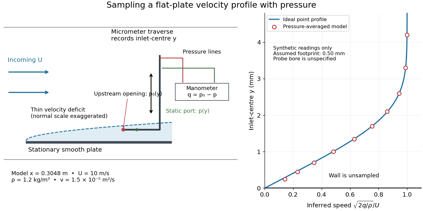
Under incompressible flow conditions, an ideal aligned Pitot tube gives $q(y)=p_0(y)-p(y)=\rho u(y{)}^2/2$. Convert the manometer head $h$ to $q=({\rho }_{\mathrm{water}}-\rho )gh$, then infer $u=\sqrt{2q/\rho }$. Here $g$ is gravitational acceleration; mass density $\rho$ can be estimated from temperature and absolute pressure using the ideal gas law. A normalized velocity profile rises from the unresolved near-wall region to a plateau, whose value defines $U$; downstream profiles should broaden and collapse when plotted against $\eta$ if the Blasius boundary layer assumptions hold. Integrating a recovered velocity profile gives displacement thickness and momentum thickness.

Additional controls for interpreting this experiment follow from the measurement model: check differential-pressure calibration with equal port pressures and known liquid heads; leak-check tubing; align the Pitot tube with the incoming velocity; convert wall contact to the inlet-centre coordinate rather than treating outside contact as $y=0$; repeat traverses and outer velocity readings to detect drift. Keep the plate smooth and aligned, and check outer static pressure at multiple downstream stations before assuming zero pressure gradient. Repeating at another station or outer velocity tests the predicted boundary-layer scaling more directly than fitting one curve. These controls are proposed checks, not actions documented as completed in the manual.

Finite probe size, wall interference, flow fluctuations, and weak near-wall dynamic pressure limit inference. Even the manual's probe-based Reynolds number criterion, ${\mathrm{Re}}_d=ud/\nu >1000$ for its ideal Bernoulli equation conversion, must be checked with local $u$, not just $U$. In the illustrative model at $x=0.3048\mathrm{m}$, ${\delta }_{99}\simeq 3.32\mathrm{mm}$; the quoted outside diameter is $2.54\mathrm{mm}$, a substantial fraction of that thickness. A real inlet's sensing footprint and correction cannot be deduced from outside diameter alone. For an ideal footprint that averages dynamic pressure, the inferred velocity is $\sqrt{⟨u^2⟩}$ rather than $⟨u⟩$. Differentiating such sparse readings to obtain wall shear stress magnifies measurement error; the momentum thickness route is less sensitive to this differentiation but still needs the unresolved near-wall contribution. The no-slip boundary condition is a model constraint here, not a direct reading from a probe centred on the wall.

A thin layer of very viscous liquid floating on an effectively inviscid denser liquid has negligible shear traction on both faces. Its leading horizontal velocity is a plug, and incompressibility gives vertical strain $w_z=-u_x$. Normal-stress balance shifts the pressure by $-2\mu u_x$, so the longitudinal excess stress is $4\mu u_x$. Combining depth-integrated momentum balance with hydrostatic reduced gravity gives the displayed extensional equations. This is distinct from a no-slip, shear-driven thin-film gravity current.

A fluid is a material that flows under sustained shear stress and cannot maintain a static shear stress in its fluid state. Liquids and gases are the usual examples. A Newtonian fluid has deviatoric stress proportional to its rate-of-strain tensor, whereas more general fluid constitutive equations can be nonlinear or have memory. In a porous medium, the fluid occupies connected voids within a load-bearing solid framework. The important distinction is the response to a continuing tangential force: an ordinary elastic solid can settle into a fixed deformation, while an ordinary fluid continues to deform. A fluid can nevertheless be at rest when no unbalanced shear stress drives it. ^[ref]

For a worked example, place a Newtonian fluid between parallel plates separated by $h=1\mathrm{mm}$, keep the lower plate fixed and move the upper one at $U=0.10\mathrm{m}{\mathrm{s}}^{-1}$. With no-slip boundary conditions, steady flow, no imposed pressure gradient and negligible edge effects, Couette flow has $u(y)=Uy/h$. For dynamic viscosity $\mu =0.001\mathrm{Pa}\mathrm{s}$, the shear stress magnitude isThe velocity gradient describes neighbouring layers sliding at different speeds. Doubling $U$ doubles the required shear stress; maintaining the same velocity keeps producing deformation, rather than fixing a final shape. This gives viscosity a concrete meaning: resistance to a rate of motion, not a prohibition on motion.

Fluid mechanics studies the motion and forces of liquids and gases. Its central simplification is the continuum approximation: replace individual molecules by bulk properties defined at every position and time. The averaging region must contain many molecules while remaining small compared with the distances over which those properties vary. A fluid element is such a small material parcel, rather than a single molecule. This connects fluid mechanics to continuum mechanics and makes calculus useful for describing flow. ^[ref]

Three basic fields are the velocity field $\mathbf{u}(\mathbf{x},t)$, the mass density $\rho (\mathbf{x},t)$ and the pressure $p(\mathbf{x},t)$. The first gives a parcel's instantaneous velocity; the second gives mass per unit volume. The pressure contributes an inward normal traction $-p\mathbf{n}$ across a surface with outward unit normal $\mathbf{n}$. Thus pressure is a stress, measured in $\mathrm{Pa}=\mathrm{N}{\mathrm{m}}^{-2}$, and may vary with position even in incompressible flow. Additional viscous stresses can act tangentially. ^[ref]

The guiding questions are what must be conserved and which forces matter. Mass conservation constrains the velocity field; momentum conservation determines its response to pressure gradients, viscosity and body forces. An incompressible flow model, a Reynolds number estimate and Bernoulli's principle answer different parts of a problem. Their appeal is that a few carefully stated assumptions can determine useful quantities before the entire velocity field is known.

With uniform thermal wind $U=\Lambda z$ above a plane boundary, write the zero-interior-potential vorticity response as ${\psi }^{\prime }=\mathrm{Re}\{A{e}^{-\mu z+i(kx+ly)}\}$, where $\mu =N\sqrt{k^2+l^2}/f$ and $f>0$. Boundary vertical velocity $ϵ\cos (kx+ly-{\omega }_{0}t)$ gives $C=N^2ϵ/(f\mu )$ and natural angular frequency $\omega =\Lambda k/\mu$. An initially zero response has $A=C(e^{-i{\omega }_{0}t}-e^{-i\omega t})/[i(\omega -{\omega }_0)]$. Its continuous resonant limit is $Ct{e}^{-i\omega t}$: forcing in phase with the boundary mode supplies energy every cycle, and linear undamped theory predicts secular growth.

Take the original sphere on the tube axis, with diagonal positive hydrodynamic resistance matrix $R_0$ and axial force $W>0$. Add a freely moving neutral sphere and extend its rigid velocity through its interior. The resulting field is admissible in the original domain, so its dissipation obeys $D>q^T{R}_{0}q\ge R_{zz}{V}_z^2$ for any finite nonoverlapping placement of the extra sphere. Since only the first sphere does external work, $D=W{V}_z$, giving the displayed bound without assuming zero transverse velocity or rotation. Strictness follows because equality would require the original nontrivial analytic flow to have zero strain throughout the added ball.

For a smooth passing encounter of a force-driven sphere with a fixed sphere, isotropy and reflection symmetry imply $\mathbf{U}=[m_{\perp }(R)I+(m_{\parallel }(R)-m_{\perp }(R))\mathbf{nn}]\mathbf{F}$. Along a force axis $X$, $U_X$ is even and the transverse velocity is odd in $X$. Uniqueness then makes the trajectory fore-aft symmetric and restores the incoming impact parameter downstream. This consequence of kinematic reversibility of Stokes flow remains valid with lubrication resistance, provided the particles remain smooth, noncontacting and subject only to the stated forces. Surface roughness and contact can invalidate these assumptions.

If $H$ is continuous, piecewise twice differentiable, and has derivative jump $[H^{\prime }]=H^{\prime }(y+)-H^{\prime }(y-)$ at $y$, then its distributional second derivative is $H_{\mathrm{reg}}^{\prime \prime }+[H^{\prime }]{\delta }_y$. If the regular part is integrable and the boundary terms vanish, two integrations by parts give the displayed asymptotic expansion by the Riemann-Lebesgue lemma. A jump $[H]$ in $H$ itself instead produces $[H]e^{-iqy}/(iq)$ at leading order. This distinguishes the different decay rates of the streamfunction and streamwise velocity in linear inviscid damping in unbounded Couette flow.

Free fall is motion under gravity alone: there is no supporting normal force, engine thrust or appreciable drag force. In the Newtonian mechanics model, a test particle of mass $m$ obeys $m\ddot{\mathbf{r}}=m\mathbf{g}(\mathbf{r})$, hence $\ddot{\mathbf{r}}=\mathbf{g}(\mathbf{r})$. The mass cancels. Bodies released at the same position with the same velocity follow the same path in this model, even if their gravitational weights differ. ^[ref]

A dropped stone is one example; a coasting satellite is another. Free fall does not require motion straight down or decreasing distance to the attracting body. An ideal circular orbit has constant radius while its velocity continually turns under centripetal acceleration. The circular orbit as continuous free fall connects the familiar drop with orbital motion.

Near a surface, treating the gravitational acceleration as constant gives a useful first prediction. Over larger heights, the inverse-square law changes the acceleration during the fall. Radial free fall from rest uses conservation of mechanical energy to account for that change exactly, within the specified Newtonian gravitational field. The contrast matters: the simplest formula is an approximation to a physical model, rather than a law with the same numerical $g$ everywhere.

History also makes the idealization tangible. Galileo's Two New Sciences (1638), Third Day, Theorem II, derives distance proportional to the square of time for uniformly accelerated motion from rest; its first corollary gives successive distances in the ratios $1,3,5,7,\dots$ over equal time intervals. This is a kinematic statement, predating the gravitational inverse-square law. ^[ref]

On Apollo 15's final lunar surface excursion, David Scott released a hammer and a feather together. The near-vacuum removed the large difference in drag force familiar on Earth. NASA's report describes their arrival together within the accuracy of the release; this demonstration illustrates the free fall prediction without establishing infinite experimental precision. ^[ref]

Take downward displacement $s$ as positive, assume a constant gravitational acceleration $g>0$, and release a point mass from rest at $s=0$. Integrating $\ddot{s}=g$ twice givesFor a downward distance $h>0$, the arrival time and speed areFor the model values $h=20\mathrm{m}$ and $g=9.81\mathrm{m}{\mathrm{s}}^{-2}$, these are approximately $2.0193\mathrm{s}$ and $19.8091\mathrm{m}{\mathrm{s}}^{-1}$. Doubling the height multiplies both quantities by $\sqrt{2}$; it does not double them. The same speed follows from the work-energy theorem, $mgh=m{v}^2/2$.

For intervals of length $\Delta t$, the successive downward displacements areThus equal spacing in time produces increasingly separated positions. This is the odd-number pattern in Galileo's result. It assumes constant acceleration and release from rest; a nonzero initial velocity adds a linear term to $s(t)$.

The approximation can be estimated for a spherical source of radius $R$ and standard gravitational parameter $\mu$. Writing $g_0=\mu /R^2$, the gravitational magnitude at height $h$ isFor $h/R\ll 1$, a Taylor expansion gives $g(R+h)/g_0=1-2h/R+O((h/R{)}^2)$. Small height relative to the source's radius makes nearly constant gravity plausible; negligible drag force remains a separate requirement.

At a flat shear-free impermeable plane, a tangential torque is reflected with opposite sign because torque is an axial vector. A parallel axial rotlet dipole therefore has an opposite signed moment at the reflected source. Its velocity vanishes at the point directly beneath the image, but its velocity gradient can turn the swimmer.