A hash compression function combines a fixed-size chaining state and one fixed-size message block to produce the next chaining state. For state width $n$ and block width $b$, a common interface isA complete iterative cryptographic hash function additionally specifies its hash initialization vector, message padding, block order and output rule. For SHA-256, the state has256bits and a block has512bits; the standard defines a64-word message schedule,64rounds and the additions producing the next eight-word state.^[ref]

Here compression is not reversible file compression. The function maps $2^{n+b}$ input pairs into only $2^n$ states. Averaged over output states, each state has $2^b$ preimages, counting zero-preimage states too. Collision resistance concerns the difficulty of finding suitable collisions, not their mathematical absence.

An original deliberately weak example makes the interface concrete. Let the state be one byte and the block be two bytes, and defineStarting from hexadecimal 6a, block 00 01 gives 6b; a following 00 02 gives 6d. But 01 00 also gives 6b from the same initial state. The interface and shrinking state size alone have supplied no cryptographic security. This toy is not an approximation to the SHA-256 round function.

The standard's feedforward in SHA-256 compression adds the incoming state words to the final working words modulo $2^{32}$. Omitting that step changes the compression function even if all64rounds were otherwise correct.^[ref] A completed message digest also includes the effect of padding and is not generally the state after an unpadded payload fragment.

A crash pulse is an acceleration time history associated with a collision. It must specify a measurement location, direction and reference frame: a vehicle structure, test platform and supported component can have different histories. NASA's 1981 aircraft-seat study explicitly described crash pulses as deceleration time histories and used them to inform crashworthiness testing.^[ref]

For one-dimensional motion, the signed area under the acceleration curve is the change in velocity:Consider two original ideal stopping pulses, both lasting $T=0.10\mathrm{s}$ and reducing velocity from $8\mathrm{m}{\mathrm{s}}^{-1}$ to zero. A constant pulse needs $a=-80\mathrm{m}{\mathrm{s}}^{-2}$. A symmetric triangular pulse that begins and ends at zero needs a peak magnitude of $160\mathrm{m}{\mathrm{s}}^{-2}$, because its area is half its peak times its duration:They have the same average acceleration but different peaks and different time histories.

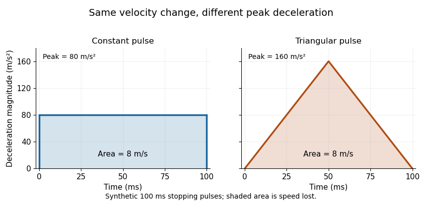
For a constant $100\mathrm{kg}$ mass following either prescribed history, Newton's second law gives the same total impulse, $m\Delta v=-800\mathrm{N}\mathrm{s}$, while the peak net force magnitude is $8000\mathrm{N}$ for the constant pulse and $16000\mathrm{N}$ for the triangular pulse. Equal pulse area therefore does not imply equal peak loading. Component motion can also differ from the motion prescribed at its support because of mechanical compliance and dynamic response.

As a historical apparatus example, the NASA study analyzed twelve light-aircraft crash tests and conducted two vertical drop tests with an energy-absorbing seat prototype at $12.8\mathrm{m}{\mathrm{s}}^{-1}$ and $36g_n$ peak deceleration, where $g_n$ denotes standard gravity. Those test conditions are distinct from the synthetic example above.^[ref]

A sulfilimine bond is a covalent sulfur–nitrogen linkage conventionally represented with an $\mathrm{S}=\mathrm{N}$ unit. In type IV collagen, it links the sulfur of a methionine side chain to the nitrogen of a hydroxylysine side chain from a neighboring protein unit. It is chemically different from a disulfide bond, which links two sulfur atoms.^[ref]

The collagen example makes atom identity important. Although hydroxylysine contains a hydroxyl group, the identified interprotein linkage involves its nitrogen, not that oxygen. Linking separate protein units reinforces the type IV collagen network of the basement membrane.

The 2009 identification combined two kinds of evidence. High-accuracy mass spectrometry constrained the composition of isolated crosslinked peptides, while nuclear magnetic resonance supplied information about the local chemical environment. Together these supported the sulfur–nitrogen assignment; mass alone would not uniquely specify how atoms of a given composition are connected.^[ref]

This is a useful example of why a protein crosslink needs a chemical description as well as a mechanical one. Observing that two protein units remain connected can establish a covalent association under the measurement conditions, but identifying the bond requires evidence about the participating atoms and their bonding environment.

The universe is the total physical system described by cosmology, including spacetime, matter and radiation. A cosmological model specifies their large-scale geometry and evolution, for example through a Friedmann-Lemaître-Robertson-Walker metric and the matter content entering the Friedmann equations.

The observable region is limited by the history of light propagation. A finite particle horizon bounds what could have sent signals to an observer since the model's early evolution; it does not imply a physical wall or establish that the entire universe is finite. Measurements of expansion, the cosmic microwave background and large-scale structure constrain the model through different physical processes.

The copolymer composition equation, also called the Mayo-Lewis equation, relates the instantaneous monomer-consumption composition to the current reacting mixture under the terminal model of copolymerization. For binary mixture mole fractions $f_1+f_2=1$, let $F_1$ be the fraction of type-1 units among the units being incorporated at that instant. Thenwhere $r_1,r_2$ are monomer reactivity ratios.^[ref] The equation concerns molar incorporation, not the mass fraction or cumulative composition of a finished specimen.

A short derivation identifies the steady-chain-end assumption. Let $c_i$ be monomer concentrations and $E_i$ concentrations of active ends. Cross-additions interconvert the end types; balancing them gives $k_{12}{E}_1{c}_2=k_{21}{E}_2{c}_1$. The two positive consumption rates areSubstitution yields $v_1/v_2=c_1(r_1{c}_1+c_2)/[c_2(c_1+r_2{c}_2)]$. Normalizing $F_1=v_1/(v_1+v_2)$ gives the stated equation. This neglects additional sources of end-type changes and uses a terminal kinetic description.

For an original example with $r_1=r_2=2$ and $f_1=0.20$, the numerator is 0.24 and the denominator is 1.68, so $F_1=1/7\approx 0.143$. The instantaneous polymer is poorer in type 1 than the available mixture. At equimolar feed the same ratios give $F_1=1/2$; this composition equality does not imply independent sequence placement.

For a finite closed batch, conversion bookkeeping for binary copolymers relates the changing monomer pool to cumulative incorporated composition. Treating an initial $f_1$ as constant after substantial selective consumption can therefore misinterpret the final sample. The IUPAC recommendation addresses conversion and integrated composition data explicitly.^[ref] Useful experiments distinguish current feed, conversion and product composition instead of treating all three as the same label.

A monomer reactivity ratio compares two propagation rate constants for the same terminal chain type in a binary copolymerization. With $k_{ij}$ denoting addition of monomer $j$ to an end of type $i$,These are homopropagation-to-cross-propagation ratios, as defined in the IUPAC terminology.^[ref] Each is dimensionless when numerator and denominator use matching rate conventions. Neither is simply the ratio of the two monomers' total consumption rates.

A chain-end addition probability depends on available concentrations as well as on the rate constants. For a type-1 end at fixed mixture mole fractions, the terminal model of copolymerization givesFor stipulated $r_1=0.5$, an equimolar mixture gives $p_{11}=1/3$. At $f_1=0.8$ it gives $p_{11}=2/3$, whereas at $f_1=0.2$ it gives $p_{11}=1/9$. Even though $k_{11}<k_{12}$ in each case, sufficient abundance of monomer 1 can make self-addition more frequent. These are illustrative kinetic parameters, not measured constants for a named commercial polymer.

The pair $(r_1,r_2)$ determines both rows of the fixed-feed transition matrix. When $r_1{r}_2=1$, its two rows coincide for nonzero feed fractions, giving independent additions within the idealized fixed-feed model. That does not require the incorporated fraction to equal the feed fraction. For example, $r_1=2$, $r_2=1/2$ and $f_1=1/2$ give probability $2/3$ of adding type 1 from either end.

Experimentally, a ratio is associated with the specified monomer pair, reaction conditions and kinetic model. It is not a universal index belonging to an isolated monomer. The IUPAC recommendation uses several starting compositions together with conversion and incorporated-composition measurements to estimate the two ratios.^[ref] One measured copolymer composition at one feed generally cannot identify two unknown ratios. Joint uncertainty and possible composition drift belong to the interpretation.

The terminal model of copolymerization represents a growing copolymer chain's addition kinetics using only the identity of its final monomeric unit. For two incoming monomers, there are two end types and four chain-growth propagation rate constants $k_{ij}$, where $i$ identifies the existing end and $j$ the incoming monomer. Earlier sequence history is omitted from this kinetic state description.^[ref]

At a fixed reacting-mixture composition, addition rates give a two-state Markov chain. With $f_1+f_2=1$ the monomer mole fractions and $r_1=k_{11}/k_{12}$, $r_2=k_{22}/k_{21}$ the monomer reactivity ratios, its transition matrix isRows label the current terminal unit; columns label the newly added unit. Each row sums to one. This interprets a sequence at fixed feed and neglects initiation, termination and feed drift over the sampled run.

For an original example, take $f_1=f_2=1/2$ and $r_1=r_2=2$. Then $P_{11}=P_{22}=2/3$ and both cross-addition probabilities are $1/3$. The stationary distribution is $(1/2,1/2)$, so the long-chain mean composition is equimolar, while equal consecutive units are favored. A run of type 1 has a geometric distribution with stopping probability $1/3$ and mean length 3. Independent equimolar placement would instead give mean run length 2. Mean composition alone does not determine sequence correlations.

The copolymer composition equation concerns the instantaneous incorporated composition implied by this model. Applying it over a finite conversion interval requires following changes in the reacting mixture. The IUPAC recommendation explicitly bases ratio estimation on conversion and composition observations at different starting feeds.^[ref]

Historically, Frank R. Mayo and Frederick M. Lewis published a 1944 theoretical comparison of monomers with a study of styrene and methyl methacrylate.^[ref] A successful terminal-model fit is evidence about a chosen kinetic representation, not proof that every chemical influence vanishes beyond the last unit.

A metal nitrosyl complex contains a coordinated nitric-oxide group, conventionally written M–NO. The metal–nitrogen–oxygen arrangement may be approximately linear or bent, and changes in geometry correlate with different bonding and reactivity.

Assigning every nitrosyl a single fixed formal charge can obscure the delocalized electronic structure. A useful counting approach groups the metal and nitrosyl together and counts the relevant electrons of that fragment. Geometry, spectroscopy and electron count then constrain one another. The original 1974 treatment explicitly relates these structural alternatives to chemical reactions.^[ref]

A metal carbonyl is a coordination complex containing carbon monoxide ligands. The ligand normally binds through carbon, donating an electron pair while accepting metal electron density into an antibonding orbital through pi backbonding.

These complementary interactions explain a useful spectroscopic test. Stronger backbonding tends to weaken the internal carbon–oxygen bond and lower its stretching frequency relative to weakly backbonded CO. A vibrational spectrum therefore probes electronic bonding, although terminal versus bridging coordination and the other ligands also affect the observed bands. Simple electron counting treats a neutral terminal CO as a two-electron donor, but that convention is not a complete description of bond strength.

Integral feedback makes a control signal depend on the accumulated tracking error. With reference signal $r(t)$ and measured output $y(t)$, introduceAt any finite equilibrium of this controller, $\dot{z}=0$ forces zero tracking error. This explains why a stable integral-control loop can reject a constant control disturbance despite an imperfect model.

For the scalar controlled plant $\dot{y}=-ay+u+d$, with constants $a,k_I>0$ and constant $r,d$, equilibrium has $y=r$ and $u=ar-d$. Perturbations satisfy ${\lambda }^2+a\lambda +k_I=0$, whose roots have negative real parts, so this particular closed loop is stable. The conclusion depends on the plant and gain: adding integration does not guarantee stability theory for an arbitrary plant. Actuator limits can also let the accumulated error grow while the requested input cannot be delivered.

Robust control designs or assesses a controller against a specified family of possible controlled plants, rather than only one nominal model. Control model uncertainty can represent uncertain parameters or unmodeled dynamics. Robust stability asks whether every allowed plant gives a stable closed loop; robust performance also requires a quantitative response criterion throughout the allowed family. Stability alone does not guarantee the required performance.^[ref]

An original scalar example makes the quantifiers explicit. Consider a controlled plant with measured state $x$ and control input $u$:The same feedback gain $k$ must be chosen before knowing $a$. Its solution is $x(t)=x(0)e^{(a-k)t}$. At the nominal value $a=2$, asymptotic stability requires only $k>2$. Choosing $k=2.5$ stabilizes that nominal model but fails at the allowed value $a=3$, where deviations grow as $e^{0.5t}$. Uniform stability over the entire closed interval instead requiresAt $k=3$, the endpoint plant has $\dot{x}=0$ and does not decay, so the strict inequality matters.

Now specify the performance bound $|x(t)|\le |x(0)|e^{-t}$ for every allowed $a$ and all $t\ge 0$. In this example it holds exactly when $k\ge 4$. Thus $k=3.1$ gives robust stability but not the requested rate of decay; the endpoint plant decays only as $e^{-0.1t}$. The performance statement is stronger than the stability statement.

The guarantee remains conditional on its model: exact state measurement, the stated parameter interval and the realizable law $u=-kx$. At $k=4$, an initial state $x(0)=2$ demands an initial input of magnitude8 in the chosen consistent units. An actuator saturation limit of5 invalidates that ideal law for this initial condition. Increasing feedback gain therefore cannot be treated as a cost-free route to robustness. A useful design specifies both the uncertainty family and the physical limits under which its guarantee is meant to apply.

A control system is an interconnection that chooses and applies control inputs to influence a controlled plant. A controller may use a reference signal, a measured output and internal state to determine those inputs. The plant, sensing, controller and input mechanism jointly determine the resulting motion. In open-loop control, the commands are chosen without updating them from the measured result; feedback control uses that result to change the commands.

An original dimensionless model shows the distinction. Let the measured output equal the plant state $x$ and let $d$ be a constant control disturbance:The open-loop command $u=r=1$ gives equilibrium $x=1+d$. A controller using both the reference command and measured tracking error can instead setSubstitution gives $\dot{x}=-(1+k)x+(1+k)r+d$. Its equilibrium and transient areWith $k=2$ and $d=0.3$, the equilibrium is1.1 instead of the open-loop value1.3. The controller reacts to the effect of the disturbance through the measured state; it need not measure $d$ separately. With no disturbance, the explicit reference term makes the equilibrium equal to1.

The interconnection matters as much as the controller formula. Measurement error changes the quantity fed back, actuator saturation can prevent delivery of the commanded input, and unmodeled dynamics can change the transient. The assumption that the entire plant state is measured is also special to this example.

Robust control asks how such a closed loop behaves across a family of possible models, distinguishing robust stability from robust performance.^[ref] A complete control-system specification therefore identifies the plant, signals, interconnection, physical limits and response criterion, rather than naming only a controller.

Dissipativity expresses an input–output balance for a dynamical system: the increase of a nonnegative storage function cannot exceed the accumulated supply rate. For state $x$, control input $u$, plant output $y$ and chosen supply rate $w(u,y)$, the requirement isfor every admissible trajectory and time interval, with $S\ge 0$. The storage function and supply rate need not be literal physical energy and power; choosing them makes a particular performance statement precise. Jan C. Willems's1972paper develops this general storage–supply formulation.^[ref]

An original mechanical example is a mass with viscous damping, driven by an applied force $u$:Choose the kinetic energy $S(v)=m{v}^2/2$ and entering power $w(u,y)=uy$. ThenIntegration gives the required inequality. The nonnegative integral $\int b{v}^{2}dt$ accounts for the mechanical energy dissipated by the damper. With no applied force, the stored kinetic energy cannot increase. A dashpot driven at constant velocity provides an experimental interpretation: supplied power is dissipated even when the mass's stored kinetic energy remains constant.

A different choice tests an input–output gain. If a storage function establishes the inequality forthen $S(x(0))=0$ and nonnegative final storage implyThe physical power balance and this squared-signal bound use the same logical structure. Neither inequality, by itself, proves that every internal state converges to zero: a hidden lossless motion can retain storage.

Behavioral systems theory describes a dynamical system by the complete set of time histories its variables are allowed to follow. With time set $\mathbb{T}$ and signal-value set $\mathbb{W}$, its behavior is a subsetAn equation specifies which functions belong to $\mathcal{B}$. It need not initially designate some variables as control inputs and others as plant outputs. Jan C. Willems emphasized physical relations and interconnection by shared variables as a motivation for this viewpoint.^[ref]

An original electrical circuit example uses two series resistors, $R_1=1\Omega$ and $R_2=2\Omega$, followed by a capacitor of capacitance $C=0.5\mathrm{F}$. Let $i$ be the common electric current, $V$ the total electric potential difference, and $v_C$ the capacitor's electric potential difference. The component laws and connection givewith the numerical equations understood in SI units. These equations define allowed histories $(V,i,v_C)$ without choosing which external variable is imposed.

Eliminating the internal variable gives, for differentiable histories,Conversely, a pair $(V,i)$ satisfying this relation can be extended by $v_C=V-3i$ to satisfy the component equations. Elimination therefore describes exactly the allowed external histories under these regularity assumptions. A prescribed initial electric charge would impose an additional initial constraint.

If the apparatus holds $i=1\mathrm{A}$ and starts with $v_C=0$, it must supply $V=(3+2t)\mathrm{V}$ with $t$ in seconds. If it instead holds $V=3\mathrm{V}$ with the same initially uncharged capacitor, the allowed electric current is $i=e^{-2t/3}\mathrm{A}$. These are different experiments on the same component relation. A chosen input–output description remains useful, but its choice follows the connection and experiment rather than being built into the definition of the physical device.

In the general framework, interconnection restricts the allowed histories by requiring designated variables to agree or satisfy connection laws. Keeping internal variables gives a component model; eliminating them gives an external description. This supports reusable models of interconnected electrical circuits, mechanical systems and other dynamical systems without assuming that every connection transmits information in only one direction.

Remaining useful life is the future time, cycle count or other usage until a component reaches a specified end-of-life criterion, conditional on its current condition and assumed future operation. The endpoint must be stated: crossing a performance limit, exhausting a discharge and reaching a long-term degradation threshold are different events. For an increasing damage variable $D$, threshold $D_c$ and present time $t$, a mathematical definition is the first-passage timeA prediction of this quantity supports condition-based maintenance, while requiring more than detection of existing damage.

For an illustrative deterministic model, let current normalized damage be0.60, the end threshold1.00 and future damage rate0.02 per hour. Linear extrapolation gives $R=(1-0.60)/0.02=20\mathrm{h}$. If the plausible future rate instead ranges from0.015 to0.025 per hour, the corresponding times range from about26.67 down to16h. Remaining useful life uncertainty therefore includes future operating conditions and degradation-model uncertainty, as well as measurement error.

A primary NASA battery-aging dataset makes the endpoint concrete. A custom testbed cycled electric batteries under controlled load and temperature, recording quantities including electric potential difference, electric current and temperature. The reported aging endpoint was30% loss of rated capacity, from2Ah to1.4Ah. That long-term endpoint is distinct from the terminal-potential threshold used to end an individual discharge.^[ref]

A useful validation compares predictions made before the endpoint with subsequently observed crossing times under documented operation. Reporting one predicted number without its endpoint, usage assumptions or uncertainty can conceal the main sources of disagreement between a model and a real endurance test.

Primary institutional physics profile. Research Interests describes nonequilibrium quantum dynamics, thermalization, quantum information and low-dimensional electronic systems. Its educational background records an MIT doctorate, and its photograph is explicitly identified as Joaquin Rodriguez Nieva. The published middle initial F. in the Raman-paper byline is retained without expansion.

Science 342(6159), 720–723 (8 November 2013), DOI 10.1126/science.1243879, first online 24 October 2013. The primary byline lists Yufeng Hao first, and includes Luigi Colombo and Rodney S. Ruoff. Abstract: surface oxygen on copper reduced graphene nucleation density; controlling it enabled centimetre-scale domains and changed growth kinetics and domain morphology. Used for the demonstrated material-growth variables, not for an unreported author-specific experimental role.

Publisher: doi.org/10.1103/PhysRevB.92.125406

Institutional repository: hdl.handle.net/1721.1/98418

Byline: Bruno R. Carvalho, Yufeng Hao, Ariete Righi, Joaquin F. Rodriguez-Nieva, Luigi Colombo, Rodney S. Ruoff, Marcos A. Pimenta, Cristiano Fantini. The publisher records publication on 8 September 2015.

Abstract: Raman bands D, G, G* and 2D were measured in graphene with differing carbon-13 concentrations and laser excitation energies; their frequency dependence on isotope mass followed a harmonic-oscillator relation.

Publisher Abstract, journals.aps.org/prb/abstract/10.1103/PhysRevB.92.125406 : the excitation-energy slopes of the G* and 2D Raman positions were unchanged across isotope concentrations; G and 2D linewidths were used to examine concentration-dependent phonon lifetimes. This is the verified abstract locator, not a reconstruction of inaccessible experimental settings.

Primary coreCIF2.4.5 definition: number of distinct sites generated by space-group symmetry, equal to general-position multiplicity divided by site-symmetry order. Companion disorder-group definition www.iucr.org/__data/iucr/cifdic_html/1/cif_core.dic/Iatom_site_disorder_group.html distinguishes jointly occupied sites within one group from alternative groups.