Topics (384k) Articles (398k) Users (410) Discussions (242) Comments (383) Files (13k) New article

The Bragg angle is the glancing angle from the incident beam to the selected lattice planes, with . If is instead the angle from the beam to the plane normal, and Bragg's law becomes . Defining the angle explicitly prevents a sine-versus-cosine error as well as a factor-of-two error in the detector deflection.
Choose and as an illustrative model, not historical measurements. For the first diffraction order,The second diffraction order has and ; the third would require and is impossible. These are different diffraction orders of the same interplanar spacing at the same wavelength.
Conversely, a first-order reflection at a measured deflection gives the interplanar spacingUsing recovers . This is the useful reversal: a known wavelength turns an angular measurement into an atomic length. An unassigned diffraction order or an unknown wavelength prevents that single measurement from determining uniquely.
2-satisfiability restricts SAT to CNF in which each Boolean clause has at most two Boolean literals. The example in Boolean satisfiability problem is therefore a 2-SAT instance. Unlike general SAT and 3-SAT, 2-SAT has a polynomial-time algorithm; its tractability concerns finding a satisfying assignment or deciding that none exists, not merely checking a candidate. 3-SAT allows up to three Boolean literals per Boolean clause and is NP-complete, even though it includes many individually easy instances such as this one.[ref]
The key logical equivalence iswhere are Boolean literals. It expresses a two-Boolean literal Boolean clause as two logical implications. Representing these logical implications as edges in a directed graph gives a route to the polynomial-time algorithm. In the example, says both and : enabling the feature requires its component, and an absent component excludes the feature.
A partial Boolean assignment gives truth values to some of a Boolean formula's Boolean variables. An extension is a complete Boolean valuation agreeing on the assigned Boolean variables. In CNF, a Boolean clause containing a true assigned Boolean literal is already satisfied; a Boolean clause whose every Boolean literal is assigned false rules out all extensions. A Boolean clause with no true assigned Boolean literal and at least one unassigned Boolean variable is unresolved. An unresolved Boolean clause need not have a compatible extension with the other Boolean clauses.
For in Boolean satisfiability problem, setting already falsifies , so both choices of can be discarded. Setting only leaves unresolved and forces if a satisfying assignment is to survive; then forces . Branching on an unassigned Boolean variable into its two truth values and discarding branches with a false Boolean clause is sound: every satisfying assignment follows one branch and cannot extend a false Boolean clause. If all branches are eliminated, the original Boolean formula is an unsatisfiable Boolean formula.
An unsatisfiable Boolean formula has no satisfying assignment. Forthe Boolean valuation falsifies the first Boolean clause, and falsifies the second. Both possible truth values fail, proving
UNSAT. Each Boolean clause alone has a satisfying assignment, but their logical conjunction does not: compatibility is the central issue. By contrast, finding just one failed Boolean valuation for a general Boolean formula only rejects that candidate. Finding one successful Boolean valuation proves SAT; proving UNSAT requires excluding every candidate, possibly with a compact argument rather than a full truth table.A satisfying assignment is a complete Boolean valuation for which a Boolean formula has truth value one, written . The notation describes a relation between the Boolean valuation and the Boolean formula. For the example in Boolean satisfiability problem, is a model of a Boolean formula , whereas is not. SAT asks for existence of at least one satisfying assignment, rather than for every Boolean valuation to work; the latter condition makes a tautology.
David H. Ackley, Geoffrey Hinton and Terrence J. Sejnowski tested their 1985 algorithm on a simulated 4–2–4 encoder. Two four-unit visible groups communicated through two hidden units, with no direct connections between the groups. Preparation set weights to zero and supplied corresponding one-active-unit patterns. Noisy clamping and annealed settling generated pair-coactivation readouts, compared with freely running readouts to choose weight changes. Learned hidden codes were the outcome. Equal sampling effort in clamped and free conditions supplied the comparison; noise limited weight growth. Finite settling was assumed to reach equilibrium, limiting the evidence for exact likelihood learning.[ref]
Take two visible bipolar units, no hidden units, zero thresholds, , and . As original training data, assign probabilities each to and and each to and . The data pair product averages to . Enumeration of all four states gives two weights and two , hence the partition function andStarting at , the positive-minus-negative difference is . A gradient ascent step of size gives . Each aligned state now has probability and each opposed state , bringing the model toward the data. The log-likelihood increases from to . Solving gives , which reproduces the data exactly. Since , this is the unique maximum. These are exact enumerations and their decimal evaluations, with no sampling or laboratory measurements.
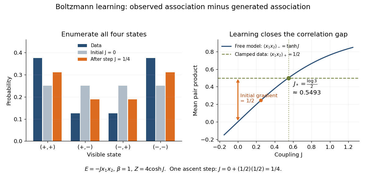
Exact probabilities and positive-minus-negative learning for two visible units
. Left: data and model probabilities before and after one gradient ascent step. Right: the data pair-product average and the model average determine the log-likelihood derivative; their intersection gives the optimal coupling. Details.Split the units into visible units , whose patterns occur in the training data, and hidden units . Let be the empirical probability distribution and maximize the average log-likelihood , where . The positive phase clamps to data and averages over ; the negative phase releases all units and averages over . The displayed difference uses these two expectations. When both units are visible, the positive pair product is supplied directly by the data.
For a proof, write . Differentiating each finite sum gives, respectively, and . Since , subtraction proves the rule. Similarly . A small positive step along these gradients increases log-likelihood. The negative term suppresses associations overproduced by the model; strengthening observed pairs alone misses this correction. The identity requires equilibrium expectations; estimates from insufficiently mixed sampling can give a biased update.
For an explosion confined approximately to a thin atmospheric layer with column mass density , an optimistic conserved-energy scaling is . The strong blast wave approximation becomes invalid near front speed , where is the ambient speed of sound, giving the displayed distance scale. Its numerical coefficient depends on the flow profiles, geometry and heat capacity ratio. Vertical energy escape makes full confinement an optimistic approximation. The criterion estimates survival of a strong shock wave, rather than whether any later acoustic wave is detectable.
Decreasing orbital period, distinct from spin slowdown. Joseph Hooton Taylor Jr. inferred masses using binary-pulsar periastron advance and binary-pulsar Einstein delay, then tested the independent period derivative against the general relativity quadrupole formula. Correcting differential Galactic acceleration gave indirect gravitational radiation evidence. This was not a terrestrial strain measurement.[ref]
In particular, the raw measured derivative schematically containsHere is positive when the source's recession accelerates. Its contribution follows by differentiating the leading Doppler effect. A decreasing observed orbital period alone therefore does not identify a unique energy-loss mechanism.
For fixed masses, binary orbital energy is and Kepler's third law gives . Positive outgoing gravitational radiation predicted by the quadrupole formula makes the orbital energy more negative, reducing and . This sign argument explains shrinking orbits, but a quantitative test also needs the predicted magnitude and orbital eccentricity dependence.
Binary-pulsar periastron advance is the gradual rotation of the orbit's argument of periapsis . A closed Kepler orbit has a fixed direction of closest approach. In general relativity, the leading conservative correction makes the relative orbit precess even before gravitational radiation causes appreciable binary-pulsar orbital decay.
For nonspinning point masses , total mass , semimajor axis of the relative orbit and orbital eccentricity , the first post-Newtonian advance per orbit isDivide by the orbital period and use Kepler's third law , where , to obtainHere is in radians per unit time. The expansion assumes .
A pulsar acts as an orbital clock: the timing delay changes as the eccentric orbit turns relative to the line of sight. If this measured advance is dominated by the relativistic point-mass term, then determine the total mass , independently of the unknown orbital inclination. They do not separately determine both component masses. A second effect, such as the binary-pulsar Einstein delay, supplies another mass relation; additional timing parameters can then test the theory instead of merely fitting it.[ref]
Spin-induced quadrupoles, tidal deformation and higher relativistic orders can contribute in other regimes and must be modeled before interpreting all observed precession as this term. At , a separate periastron direction is undefined. Advance of this direction is conceptually distinct from decreasing : conservative precession by itself is not evidence of radiated orbital energy.
The semimajor axis of the pulsar's orbit about the binary barycenter, projected along the line of sight and divided by the speed of light. The orbital inclination is zero for a face-on orbit. Thus is a time, often quoted as the numerical number of light-seconds in , not the true binary separation. The relative-orbit semimajor axis is instead ; conservation of momentum gives .
Combining Kepler's third law with that barycenter relation gives the timing form of the binary mass function, also valid for eccentric Kepler orbits:Choose and for an original example: and , where is a solar mass. For a specified pulsar mass , the smallest allowed companion mass occurs at and is approximately . A different assumed changes this bound. One measured does not determine both masses and orbital inclination.
Russell Alan Hulse and Joseph Hooton Taylor Jr. discovered this binary pulsar at Arecibo in 1974; their January 1975 paper reports a roughly pulse period and orbital period. Its unseen companion was not detected as a second radio pulsar. Discovery of the orbit preceded the later binary-pulsar orbital decay test.[ref]
Discovery of a Pulsar in a Binary System by Russell Alan Hulse and Joseph Hooton Taylor Jr.. Discovery of a Pulsar in a Binary System, 15 January 1975, L51 opening and section II; L53 section IV
The 1993 Nobel Prize in Physics recognized the discovery.[ref]
All Nobel Prizes in Physics by Nobel Prize Outreach. 1993 entry, joint award and discovery motivation
A Kondo insulator has a bulk insulating state associated with mixing between relatively localized correlated electronic states and itinerant conduction states. A renormalized two-band picture captures a narrow hybridization gap, although an uncorrelated orbital-mixing model does not explain the formation and temperature dependence of the coherent low-energy state. Samarium hexaboride is an example.
Suppose the exterior of a sphere also has zero Dirichlet boundary conditions on the part of its equatorial plane outside the sphere. The plane separates the upper and lower domains. Extend the sphere data of each hemisphere oddly across the equator, and apply the axisymmetric harmonic extension from a sphere separately to these two odd extensions. Only odd-degree Legendre polynomials occur, and every such polynomial vanishes at . Thus the resulting harmonic function vanishes on the plane. For upper data on , the exterior coefficients are for odd . If , the plane and sphere data agree at their shared edge. The same construction with the lower data gives the lower solution; their normal derivatives need not match through a conducting sheet.
A narrow fringe makes the center easier to resolve statistically; it does not certify an unbiased frequency. For example, with ideal pulses and a second-pulse oscillation phase offset , the finite-pulse Ramsey transition probability approachesThis sign uses exactly the Rabi detuning convention and pulse Hamiltonian operator above, with the second pulse replacing by . The factor converts angular frequency to ordinary frequency. For the original example, rad and give a shift of about . For finite pulses or distributed flight times, use the full signal and its atomic clock frequency lock rather than inserting an unweighted mean .
NIST-7 used optical pumping and fluorescence. Controls included field-sensitive transitions, independent beam-speed measurements, microwave power stabilization, and beam reversal for cavity quantum phase errors.[ref]
Primary Atomic Frequency Standards at NIST by D. B. Sullivan and others. §2.2, pp. 50–52: optical readout and frequency-shift controls
The connection to special relativity is quantitative. A freely moving emitter's proper time advances more slowly than laboratory time by . With first-order propagation effects removed in the ideal comparison, its internal laboratory frequency is thereforeCorrecting an ensemble signal requires the effective velocity weights of preparation, interrogation and detection, not simply the oven's mean speed. Additional shifts from Zeeman splitting, unwanted light, collisions and cavity fields likewise require separate evaluation; feedback control locks to the observed line, including any uncorrected bias. Comparing clocks at different gravitational potentials additionally requires gravitational time dilation. The moving-clock experiments in twin paradox clock experiments compare calibrated clock readings along different world lines; the beam atoms' internal motion is part of the clock mechanism's own correction.
A peak has zero slope at its center, so a single peak-height reading does not tell feedback control which way to tune. Instead sample the two sides at ordinary frequencies , where is a chosen modulation offset, and subtract:For an even signal around the true center , write . A Taylor expansion gives . On the descending side of a positive central peak , so the update has restoring sign for and is locally stable in this ideal discrete update when . A detector dip requires the opposite sign. These conditions follow from linearizing the update, not from assuming any particular electronics.
For the ideal signal , choose . Then . With and , a center error of gives exact . The sign directs the update toward lower frequency. Constant background cancels, but background drift between samples or asymmetric neighboring spectral lines can bias the zero. An initial scan matters because other fringes can also supply zeros.
An oven supplies a collimated caesium beam. State-selecting magnets precede and follow two coherent microwave interaction regions; a weak static magnetic field separates sublevels. The clock transition connects and . Transferred atoms reach a heated ionizing collector. A detector scan identifies the resonance before locking.[ref]
The Physical Basis of Atomic Frequency Standards by A. S. Risley. April 1971 edition, §5.3, pp. 36–38, Fig. 7
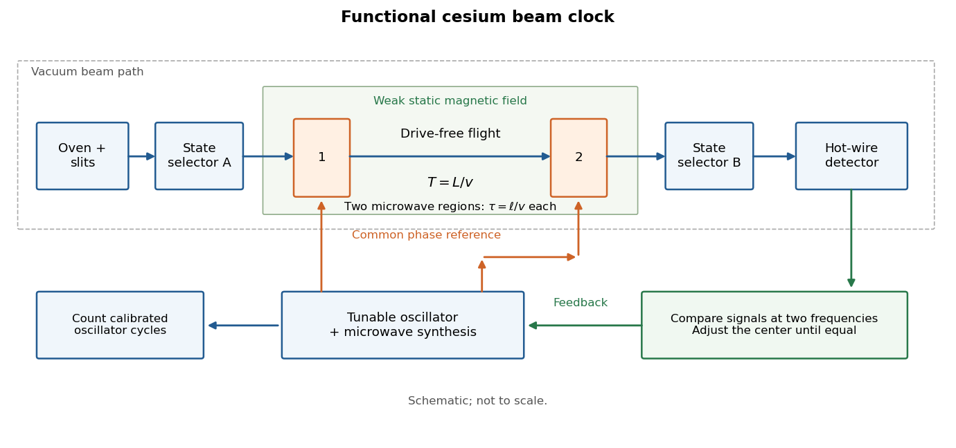
Here labels the total angular momentum and its projection. The selected pair is a two-level system inside a larger set of atomic energy levels; treating every oven atom as a prepared qubit would overstate the preparation. A measured detector signal may be modeled as , with background and gain . Background subtraction and stable transmission are necessary before interpreting the signal as a transition probability. The velocity-averaged Ramsey line provides one explicit ideal example; its chosen dimensions are not historical specifications.
The fixed-target production threshold concerns the incident accelerator beam, whereas antiproton mass from momentum and velocity concerns an outgoing secondary beam. To see the distinction, consider a free proton hitting a stationary free proton, producingThe final electric charge is and final baryon number is , as initially. Approximate all four final rest masses by the same proton rest mass . With metric signature , define the squared centre-of-mass energy by . The incident proton has total energy , and the target four-momentum is . Four-momentum conservation and the mass shell relation giveAt threshold the four final particles have zero relative momentum in their centre-of-momentum frame, so . HenceOnly of new rest energy is created. The larger incident kinetic energy is required because the final system must also carry the initial laboratory momentum. The incident total energy at threshold is ; neither this nor is the selected secondary momentum.
The 1955 authors explicitly qualified the stationary-nucleon threshold: target nucleon motion inside an atomic nucleus can lower the required incident energy.[ref]
The kinematic reason is visible for two on-shell incoming nucleons:A target momentum directed against the beam increases . Applying this illustration to a bound nucleon also requires binding energy and residual-nucleus recoil; the free stationary-target result is therefore not a universal sharp threshold for a copper target. A low observed secondary momentum is entirely compatible with a much larger accelerator kinetic energy.
Pinned article: Introduction to the OurBigBook Project
Welcome to the OurBigBook Project! Our goal is to create the perfect publishing platform for STEM subjects, and get university-level students to write the best free STEM tutorials ever.
Everyone is welcome to create an account and play with the site: ourbigbook.com/go/register. We belive that students themselves can write amazing tutorials, but teachers are welcome too. You can write about anything you want, it doesn't have to be STEM or even educational. Silly test content is very welcome and you won't be penalized in any way. Just keep it legal!
Intro to OurBigBook
. Source. We have two killer features:
- topics: topics group articles by different users with the same title, e.g. here is the topic for the "Fundamental Theorem of Calculus" ourbigbook.com/go/topic/fundamental-theorem-of-calculusArticles of different users are sorted by upvote within each article page. This feature is a bit like:
- a Wikipedia where each user can have their own version of each article
- a Q&A website like Stack Overflow, where multiple people can give their views on a given topic, and the best ones are sorted by upvote. Except you don't need to wait for someone to ask first, and any topic goes, no matter how narrow or broad
This feature makes it possible for readers to find better explanations of any topic created by other writers. And it allows writers to create an explanation in a place that readers might actually find it.
Figure 1. Screenshot of the "Derivative" topic page. View it live at: ourbigbook.com/go/topic/derivativeVideo 2. OurBigBook Web topics demo. Source. - local editing: you can store all your personal knowledge base content locally in a plaintext markup format that can be edited locally and published either:This way you can be sure that even if OurBigBook.com were to go down one day (which we have no plans to do as it is quite cheap to host!), your content will still be perfectly readable as a static site.
- to OurBigBook.com to get awesome multi-user features like topics and likes
- as HTML files to a static website, which you can host yourself for free on many external providers like GitHub Pages, and remain in full control

Figure 2. You can publish local OurBigBook lightweight markup files to either OurBigBook.com or as a static website.
Figure 3. Visual Studio Code extension installation.
Figure 5. . You can also edit articles on the Web editor without installing anything locally. Video 3. Edit locally and publish demo. Source. This shows editing OurBigBook Markup and publishing it using the Visual Studio Code extension. 
- Infinitely deep tables of contents:




All our software is open source and hosted at: github.com/ourbigbook/ourbigbook
Further documentation can be found at: docs.ourbigbook.com
Feel free to reach our to us for any help or suggestions: docs.ourbigbook.com/#contact