Topics (384k) Articles (398k) Users (410) Discussions (242) Comments (383) Files (13k) New article

The median eminence is a region at the base of the hypothalamus where neurosecretory terminals release regulatory hormones near the first capillary bed of the hypophyseal portal system. It is an interface between hypothalamic neurons and the vascular route to the anterior pituitary. A GnRH terminal here is a site of release; the neuron's soma need not occupy the same location.[ref]
Vascular endothelial cells promote acute plasticity in ependymoglial cells of the neuroendocrine brain by Sandrine De Seranno and others. Introduction and Abstract: median-eminence neurosecretory interface
Access to the capillaries also depends on neighboring glial cells, including tanycytes. In a 2004 study, female-rat tissue containing the median eminence was incubated for 30 minutes with or without added arginine, a substrate for nitric oxide production. Immunoelectron microscopy identified GnRH-containing terminals. In treated preparations, the investigators observed structural changes bringing terminals into direct contact with the space beside the capillaries. Complementary cell-culture experiments implicated signals from endothelium in glial remodeling.[ref]
Vascular endothelial cells promote acute plasticity in ependymoglial cells of the neuroendocrine brain by Sandrine De Seranno and others. Abstract; Figure7:500micromolar L-arginine,30min and immunogold localization
The comparison is illuminating because the route is more than a fixed pipe connecting two glands. The arrangement of neurons, glial cells and blood vessels can alter access to the release surface. A microscopic structural observation and a measurement of circulating hormone nevertheless remain different kinds of evidence: proximity alone does not quantify how much GnRH enters the blood.
Hot-wire anemometry is the measurement method that turns a hot-wire anemometer's heat-transfer signal into a flow velocity time series and its statistics. It is especially useful for resolving fluctuations, but the interpreted quantity depends on probe direction, spatial extent and dynamic response. The manufacturer's primary method requires known-flow calibration and separately describes directional and temperature sensitivity.[ref]
Measurement Principles of CTA by Dantec Dynamics. Velocity sensitivity, Directional sensitivity and Temperature sensitivity
The order of processing matters because a nonlinear calibration does not commute with averaging. For an original relation in numerical volts and metres per second, equal-duration speeds and give outputs and . Converting their average output giveswhereas converting each output first and then averaging gives the true two-level mean . A proposed processing chain therefore applies the validated instantaneous conversion before calculating statistics, subject to its bandwidth and direction limitations.
For equally spaced converted samples, define the record mean and root-mean-square fluctuation byThe stipulated record has mean and . Its ratio is about . This is the RMS fluctuation of that finite record, not automatically an unbiased estimate based on four independent observations; turbulence samples can be strongly correlated.
The measurement has both temporal and spatial filters. An electronic anti-aliasing filter must sufficiently attenuate unresolved fluctuations before digitization; a sampling rate of has Nyquist frequency regardless of the wire's faster response. Finite wire length produces hot-wire spatial averaging, so increasing sampling rate alone cannot recover spatial scales already averaged by the sensor. Flow direction changes can also be misread as speed changes by a single-wire calibration.
A useful proposed grid-turbulence experiment keeps the wire transverse to a positive mean flow, performs a reference-flow calibration before and after acquisition, records ambient temperature, and documents wire geometry, bridge settings, sample rate and filtering. Compare means and fluctuation spectra at different positions and repeat with a shorter wire or a changed electronic bandwidth. A changed high-frequency spectrum can reflect instrumental filtering as well as changed flow physics.
The electrical control loop should also be characterized rather than assigning a universal bandwidth to the wire alone; the primary description explicitly connects frequency response to wire and servo behavior.[ref] A measured time series is evidence for the flow only within the direction, spatial, thermal and frequency ranges actually tested.
A constant-temperature hot-wire anemometer is a hot-wire anemometer whose electrical feedback adjusts wire heating to keep a chosen wire resistance approximately constant. The resistance acts as a temperature indicator; increasing flow cooling calls for increased electrical power. The primary manufacturer's arrangement places the wire in a Wheatstone bridge controlled by a servo amplifier.[ref]
A simple resistance-temperature calibration illustrates the setpoint. If the cold resistance at fluid temperature is , approximateFor stipulated , and , the overtemperature is . At ambient , that corresponds to wire temperature in this linear model. These parameters are illustrative, not universal tungsten specifications. A fixed resistance setpoint and a fixed overtemperature require different adjustments when ambient temperature changes.
At steady state, the heating balances convective, support-conduction and radiative losses. The observed bridge output must be calibrated against known flow with the same probe, fluid and operating conditions. A bridge output squared may follow an empirical relation over a limited range, but circuit ratios and losses matter before identifying that output with wire power. The manufacturer's technical account separately treats velocity, directional and temperature calibration.[ref]
Measurement Principles of CTA by Dantec Dynamics. Velocity sensitivity, Directional sensitivity and Temperature sensitivity
Finite-bandwidth thermal feedback in hot-wire anemometry can be explored with an original local model. Let a temperature perturbation satisfywhere is wire heat capacity, a linearized thermal-loss coefficient and the incremental cooling per speed change. An ideal proportional power controller applies , with . HenceA cooling perturbation first lowers temperature, causing the controller to raise power. Finite feedback gain leaves a residual temperature perturbation and gives DC power sensitivity .
For , and , the model's thermal time constant changes from to and its half-power frequency from about to . The closed-loop DC response is . This calculation assumes an instantaneous controller; real amplifier and cable dynamics can add phase lag and limit usable gain.
A proposed characterization calibrates the steady speed response, then applies a small electrical test perturbation and examines settling and ringing while measuring ambient temperature. Check the response over the intended flow range and verify that the measuring electronics do not clip. The primary practical guide describes the feedback bridge as part of the complete measuring chain.[ref]
How to measure turbulence with hot-wire anemometers - a practical guide by Finn E. Jørgensen. §15.5, printed p. 51
A fast electrical response alone does not establish spatial resolution or uniquely determine the direction of a reversing flow.The Horvitz-Thompson variance estimator estimates the sampling variance of a Horvitz-Thompson estimator using observed values and known individual and joint inclusion probabilities. It is a random estimate of a fixed design-dependent variance, rather than the variance itself.
Let be an inclusion indicator, , and , with . For fixed population values , write . Bilinearity of covariance givesUnder pairwise inclusion positivity, a sample provides the estimatorThe diagonal terms are included. Taking expected values replaces by 1, proving . This is the pairwise counterpart of inverse-probability expansion for the finite population total.[ref]
An original exact example uses fixed values . Select with probabilities , respectively. Then , and the possible total estimates are . Their expected value is the true total 4, with varianceFor those same samples, the variance estimates are . Their expected value is also 2. In particular, for , the two diagonal contributions are 4 and 2, while the combined off-diagonal contribution is , giving .
Thus this unbiased estimator of variance can be negative in a realized sample. Replacing a negative result by zero changes its expected value; in this example that modification raises the mean estimate to . A positive square root is therefore not always available as a sample standard error from this particular formula. If some , dropping an unobservable cross-product does not preserve the proof; the missing term needs separate analysis.
Homogeneity-study measurement-order confounding occurs when container identity is associated with measurement time, so that instrumental drift can appear to be a difference between portions of a reference material. It is a sampling-design problem in a homogeneity study with replicated test portions: repeating each container twice does not by itself separate its material effect from the instrument's time dependence.
An original measurement model adds a drift term to the container and residual effects:Here is the container contribution, a linear drift rate and the observation time. A one-way analysis of variance that omits time can assign part of to container variation. This is confounding, rather than evidence that the material actually changed composition.
Suppose three identical containers have true value 100 in a chosen unit, residual noise is absent, and the instrument increases by one unit per measurement interval. Measuring A twice, then B twice, then C twice at times 0 through 5 produces pairs , and . Their means are 100.5, 102.5 and 104.5. The within-container mean square is and the between-container mean square is . The usual two-replicate estimate givesalthough the stipulated true between-container variance is zero. These are invented observations showing an omitted effect, not a fitted material certificate.
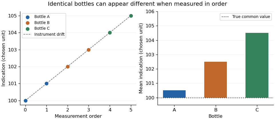
Original example: sequential measurements of identical bottles inherit an instrument's linear drift
. Details. Randomization breaks the systematic link between container label and measurement order in the design, but one random sequence does not guarantee cancellation of drift. The IUPAC protocol requires randomized analytical order and inspection for suspicious trends in the resulting data.[ref]
The International Harmonized Protocol for the proficiency testing of analytical chemistry laboratories by Michael Thompson and others. Appendix 1, A1.1 and A1.3, printed pp. 177–179; §3.11.4
A deliberately balanced illustration assigns A to times 0 and 5, B to 1 and 4, and C to 2 and 3. Each mean then contains the same linear-drift contribution, . This cancels drift from differences of those means, but does not reproduce the independent, equal-variance residual model: the within-pair differences still contain drift. Nonlinear drift would also require further assessment.
Retain timestamps, sample identities and the planned order. Suitable experimental blocks, repeated control measurements or a justified drift-aware homogeneity analysis can help distinguish instrument behaviour from material variation. A small residual scatter within adjacent duplicates is insufficient evidence that the instrument stayed stable over the full study.
H3K27 methylation is addition of one or more methyl groups to the side chain of lysine 27 in histone H3. Mono-, di- and trimethylated states are different chemical states; a measurement of one is not automatically a measurement of the others. H3K27 trimethylation is particularly associated with Polycomb-mediated gene silencing. [ref]
A mechanistic test distinguishes correlation from catalysis. A purified complex can be supplied with histones and a methyl donor to test transfer, while changing a catalytic region tests whether that activity depends on an intact enzyme. In a cell, the distribution of the mark also depends on recruitment, removal and replacement of histones, not only on total enzyme abundance.
A heavy-atom derivative is a modified crystal containing ordered heavy-atom sites that can provide a reference scattering contribution for X-ray crystallography. The crystal before modification is called native. For single isomorphous replacement or multiple isomorphous replacement, the desired crystal isomorphism means that the parent crystal structure is sufficiently preserved for its contribution to be shared between data sets. Merely detecting the added chemical element does not establish that model.
The early myoglobin work provides an experimental example. Several crystals with mercury or gold at single sites on the protein were compared with unsubstituted crystals to infer phases. These are chemically modified reference specimens, not computational substitute structures.[ref]
Structure of Myoglobin: A Three-Dimensional Fourier Synthesis at 2 Å. Resolution by J. C. Kendrew and others. p422, opening paragraph on the earlier6Å analysis
Crystallographic site occupancy describes the fraction present at a modeled site. The IUCr heavy-atom dictionary defines an occupancy separately for each site and derivative.[ref]
Heavy-atom site occupancy in the PDBx/mmCIF Dictionary. item
In a simplified single-site model with fixed position and displacement behavior, let be the full-occupancy complex amplitude and let be occupancy. ThenFor an original illustrative reflection, choose and . With , the derivative amplitude is and its squared magnitude is58. At full occupancy it is and its squared magnitude is109. The native squared magnitude is25. Thus doubling occupancy doubles this modeled heavy-atom amplitude, but does not generally double the measured intensity change: interference with the parent contribution matters._phasing_MIR_der_site.occupancyUseful derivative assessment therefore concerns ordered scattering and comparability as well as chemical uptake. If modification changes the parent structure substantially, the assumed decomposition into unchanged parent plus added reference is inadequate. Heavy-atom labeling describes the motivation for introducing the reference; a heavy-atom derivative is the resulting experimental specimen.
Single isomorphous replacement estimates phases in X-ray crystallography by comparing a native crystal with one heavy-atom derivative. Under the ideal crystal isomorphism assumption, a reflection's derivative structure factor is , where the heavy-atom model supplies the complex reference . The measured magnitudes constrain to two circles in the complex plane: one centered at zero with radius , the other centered at with radius . A general intersection gives two phase choices.[ref]
Phasing diagrams in CCP4 Basic Maths for Protein Crystallographers. SIR, two-circle construction
An original exact example uses , real and positive, and . Writing givesSubtracting the equations gives , hence and . The alternatives areBoth alternatives predict exactly the same native and derivative intensities. Greater precision in these two magnitudes alone cannot select between them. The phase is the missing direction of a complex amplitude, not an unmeasured additive intensity.
Multiple isomorphous replacement can supply an additional circle from another derivative. The numerical example there resolves these particular candidates. In actual measurements, uncertainty, imperfect crystal isomorphism and an imperfect heavy-atom model broaden the constraints, so exact circle crossings are an explanatory idealization.
Multiple isomorphous replacement combines a native X-ray diffraction data set with data from two or more heavy-atom derivatives to estimate the native structure factor phases. In the ideal crystal isomorphism model, each derivative adds a constraint . Consistently referenced heavy-atom models can distinguish the two alternatives left by single isomorphous replacement.[ref]
Phasing diagrams in CCP4 Basic Maths for Protein Crystallographers. MIR, third circle and matching origin/hand
Continue the original example in single isomorphous replacement, where both fit the native amplitude5 and first derivative with . Choose a second reference . Its predicted squared amplitudes differ:A measured second-derivative amplitude therefore selects in this exact model. If the second reference had instead been real, both candidates would still have equal magnitudes after adding it. An additional derivative must contribute useful geometry, rather than merely repeat a constraint.
The heavy-atom models must share a consistent coordinate origin and handedness. Resolving a circle-crossing ambiguity does not by itself determine absolute handedness: conjugating all the amplitudes preserves their magnitudes. CCP4's diagrams explicitly retain this distinction.[ref]
Phasing diagrams in CCP4 Basic Maths for Protein Crystallographers. MIR, conjugate phases and enantiomorphic maps
The method has a concrete experimental history. The opening of the1960 myoglobin structure report describes several mercury- or gold-containing derivatives whose X-ray diffraction patterns were compared with the unsubstituted protein. These measurements had supplied phases for the earlier map at spacings greater than6Å; the new report advanced the analysis to2Å.[ref]
Structure of Myoglobin: A Three-Dimensional Fourier Synthesis at 2 Å. Resolution by J. C. Kendrew and others. p422, opening paragraph
Different labeled crystals supplied information unavailable from native intensities alone.The core of an index- handle is the disk . Its boundary is the attaching sphere. The complementary disk is the cocore, whose boundary is the belt sphere.
The core records the new -dimensional direction introduced by handle attachment. Core and cocore meet transversely at the single center point, with complementary dimensions and . This intersection explains their dual roles in handle descriptions and cancellation arguments.
For a three-dimensional one-handle , the core is an arc joining the two attaching disks, while the cocore is a cross-sectional two-disk. Cutting across the cocore and tracing along the core therefore describe different geometric operations. The full handle is an -dimensional thickening of its core, not just the core disk itself.
For an additive left -module , a two-coboundary is a degree-two group cochain obtained from a degree-one cochain byIt is automatically a two-cocycle because . Expanding the four terms in makes every contribution cancel.
For trivial action and , take and . Then , a nonzero cochain representing the zero class in . Being cohomologically trivial does not require being pointwise zero.
Changing a section in an abelian-kernel group extension changes its extension cocycle by a two-coboundary. This is the mechanism behind quotienting two-cocycles by two-coboundaries when defining second group cohomology.
The center of a graph is the set of vertices with minimum graph eccentricity. For a finite connected graph , putHere is shortest-path distance and is the graph radius. The center solves a facility-placement problem in which the cost is the distance to the farthest vertex.
In a five-vertex path graph, eccentricities are , so only the middle vertex is central. In a four-vertex path, the two middle vertices both have eccentricity two. The center of a tree is always a single vertex or a pair of adjacent vertices: repeatedly deleting all leaves exposes its middle. For a general graph the center need not have this form; every vertex of a cycle graph is central.
Two graphs exhibit graph non-isomorphism when no bijection of their vertex sets preserves and reflects adjacency. For finite simple graphs and , this means there is no bijection satisfyingfor every pair of distinct vertices. Changing vertex names or drawing positions cannot establish non-isomorphism; the adjacency structure must differ.
A graph invariant is a property preserved by graph isomorphism. Different numbers of vertices, edges or connected components of a graph immediately prove non-isomorphism. Equal values of one invariant need not prove isomorphism.
For an original example, let be the six-vertex cycle graph with edges , and let be the disjoint union of graphs consisting of triangles and . Both have six vertices, six edges and degree sequence . Nevertheless, is a connected graph, whereas has two connected components. Any adjacency-preserving bijection transports a path to a path, so it would have to preserve connectedness. No such bijection exists. The common degree sequence is therefore an incomplete isomorphism test.
Finite exhaustive checking provides a direct decision procedure: if the vertex counts agree at , examine each of the possible bijections and test adjacency. If every bijection fails, the graphs are non-isomorphic. More efficient procedures can avoid enumerating all bijections; this simple procedure explains the logical criterion, rather than a practical performance bound.
Software tests also require a decision about what belongs to the structure. NetworkX's
is_isomorphic ignores node and edge attributes by default; matching functions can require them to agree.[ref]is_isomorphic documentation by NetworkX. node_match, edge_match and Examples
Two differently colored copies of the same uncolored graph can thus be isomorphic as simple graphs but non-isomorphic under a color-preserving requirement. The intended graph category must be specified before interpreting a negative result. Pinned article: Introduction to the OurBigBook Project
Welcome to the OurBigBook Project! Our goal is to create the perfect publishing platform for STEM subjects, and get university-level students to write the best free STEM tutorials ever.
Everyone is welcome to create an account and play with the site: ourbigbook.com/go/register. We belive that students themselves can write amazing tutorials, but teachers are welcome too. You can write about anything you want, it doesn't have to be STEM or even educational. Silly test content is very welcome and you won't be penalized in any way. Just keep it legal!
Intro to OurBigBook
. Source. We have two killer features:
- topics: topics group articles by different users with the same title, e.g. here is the topic for the "Fundamental Theorem of Calculus" ourbigbook.com/go/topic/fundamental-theorem-of-calculusArticles of different users are sorted by upvote within each article page. This feature is a bit like:
- a Wikipedia where each user can have their own version of each article
- a Q&A website like Stack Overflow, where multiple people can give their views on a given topic, and the best ones are sorted by upvote. Except you don't need to wait for someone to ask first, and any topic goes, no matter how narrow or broad
This feature makes it possible for readers to find better explanations of any topic created by other writers. And it allows writers to create an explanation in a place that readers might actually find it.
Figure 1. Screenshot of the "Derivative" topic page. View it live at: ourbigbook.com/go/topic/derivativeVideo 2. OurBigBook Web topics demo. Source. - local editing: you can store all your personal knowledge base content locally in a plaintext markup format that can be edited locally and published either:This way you can be sure that even if OurBigBook.com were to go down one day (which we have no plans to do as it is quite cheap to host!), your content will still be perfectly readable as a static site.
- to OurBigBook.com to get awesome multi-user features like topics and likes
- as HTML files to a static website, which you can host yourself for free on many external providers like GitHub Pages, and remain in full control

Figure 2. You can publish local OurBigBook lightweight markup files to either OurBigBook.com or as a static website.
Figure 3. Visual Studio Code extension installation.
Figure 5. . You can also edit articles on the Web editor without installing anything locally. Video 3. Edit locally and publish demo. Source. This shows editing OurBigBook Markup and publishing it using the Visual Studio Code extension. 
- Infinitely deep tables of contents:



All our software is open source and hosted at: github.com/ourbigbook/ourbigbook
Further documentation can be found at: docs.ourbigbook.com
Feel free to reach our to us for any help or suggestions: docs.ourbigbook.com/#contact