Topics (384k) Articles (398k) Users (410) Discussions (242) Comments (383) Files (13k) New article

A graph invariant assigns a value to a graph in a way preserved by graph isomorphism. For an invariant ,The value may be a number, a sequence or another mathematical object whose equality has been specified. Isomorphism preserves adjacency while allowing a relabeling of vertices; a drawing's page coordinates are therefore not a graph invariant.[ref]
Examples include vertex count, edge count, the sorted degree sequence and the number of connected components of a graph. If even one invariant differs, it proves graph non-isomorphism. Equality of an invariant usually supplies only a necessary condition. For example, a six-vertex cycle graph and two disjoint triangles both have six vertices, six edges and six degrees equal to2, but only the cycle is a connected graph. The example in graph non-isomorphism proves the obstruction through connectedness.
The adjacency matrix gives an algebraic way to construct invariants. Relabeling a graph replaces by for a permutation matrix . HenceFor a finite undirected simple graph, the th diagonal entry of counts three-step closed walks from vertex . Every triangle gives two traversal directions and three possible starting vertices, so the number of triangles in a graph isThe six-cycle has no triangles and trace zero; two disjoint triangles have trace12 and triangle count2. This invariant distinguishes them even though their degree sequences agree.
A complete graph invariant would satisfy the reverse implication too: equal values would guarantee graph isomorphism. Being easy to compute and being complete are separate properties. Combining several inexpensive invariants can reject many non-isomorphic pairs, but a surviving pair still requires a justification that the chosen information determines its adjacency structure.
Primary graft patency measures how long a graft remains open without an intervention that terminates the primary-patency endpoint. It concerns the history since the original reconstruction, not merely whether a bypass graft is open on today’s image. Under the 1997 reporting standard, work confined to disease beyond the graft and its anastomosis can be an exception; an intervention on the graft to prevent its failure is not.[ref]
Recommended standards for reports dealing with lower extremity ischemia: Revised version by Robert B. Rutherford and others. Printed p. 525, primary-patency definition and native-vessel exceptions
For an explicit time-to-event model, define as the first qualifying loss of primary patency. Its survival function isOpening a narrowed but still patent graft by a qualifying preventive procedure can end primary graft patency even though blood never stopped flowing. Later rescue does not put that same graft back into the original primary-patency history. Assisted primary graft patency and secondary graft patency answer different questions about preserving or restoring function.
An original five-graft example demonstrates the denominator. All enter follow-up together. One has a qualifying intervention at month 2, another is last observed event-free at month 3, and a third occludes at month 4; the other two remain event-free through month 4. The Kaplan–Meier estimator givesThe graft patency risk set falls after both the first endpoint and the later right censoring. The censored graft is neither declared a failure nor assumed patent indefinitely. Interpreting this estimate requires an appropriate independent-censoring assumption.
A report should identify the original procedure date, qualifying interventions, documented occlusions and observation limits. A status image alone cannot reconstruct every earlier event. Primary graft patency is therefore most informative alongside the intervention history and separately defined clinical outcomes, rather than as an unexplained percentage.
Assisted primary graft patency credits maintenance of an open graft by interventions performed before it occludes. The distinction is temporal: assistance preserves uninterrupted patency, whereas successful reopening after an occlusion belongs to secondary graft patency. The 1997 reporting standard introduced this distinction explicitly when revising how preventive graft procedures were counted.[ref]
Recommended standards for reports dealing with lower extremity ischemia: Revised version by Robert B. Rutherford and others. Printed p. 525, assisted-primary-patency discussion
A qualifying preventive intervention can end primary graft patency without ending assisted primary graft patency. Thus the two endpoints measure different aspects of durability: the former concerns performance without that assistance, while the latter also credits preservation work. They should share a stated time origin and compatible rules before their curves are compared.
Consider an original four-graft cohort. At month 2, one graft undergoes a preventive procedure while still open. At month 3, a different graft occludes, then is successfully reopened at month 4. The other two remain open without procedures. With complete follow-up to month 4, primary patency is , assisted primary patency is , and secondary patency is , assuming the restoration qualifies for the original reconstruction’s secondary endpoint. The reopened graft does not regain an uninterrupted assisted-primary history.
Surveillance influences what is observed and when assistance is undertaken. A narrowing may be detected before occlusion, so reports need their detection and intervention rules. A high assisted-primary proportion can coexist with many preventive procedures; it is not a measure of low procedural burden. Conversely, two cohorts with different surveillance intensity are not made directly comparable merely by using the same endpoint name.
With incomplete follow-up, survival analysis uses a graft patency risk set rather than treating every graft as observed to the final study date. Clinical interpretation also requires the separately measured consequences for tissue function and the patient. Preserving a conduit is an important intermediate outcome, not a complete description of benefit.
Secondary graft patency credits continued function of the original graft reconstruction, including qualifying restoration after an occlusion. It differs from assisted primary graft patency, which requires that patency never have been lost. The 1997 reporting standard limits what counts as salvaging the original reconstruction: a replacement that does not preserve the required original graft continuity is not simply a continuation of its secondary patency.[ref]
Recommended standards for reports dealing with lower extremity ischemia: Revised version by Robert B. Rutherford and others. Printed p. 525, secondary patency and redo-reconstruction rules
Secondary patency is a durability endpoint that can credit successful salvage. It does not assert that blood flowed continuously during an interval in which the graft was occluded. An instantaneous graft patency assessment and a reconstructed follow-up history therefore need not be the same data object.
An original example follows five grafts through six months. One occludes at month 2 but is successfully reopened at month 3 with a qualifying salvage of the original reconstruction. Another occludes at month 4 and is not restored. The remaining three stay patent without procedures. At the end of this complete observation period, retain secondary patency while only have uninterrupted patency without a qualifying intervention. A newly created replacement bypass should be recorded under the stated reconstruction rules, rather than silently resetting the old graft’s clock.
A time-dependent analysis must define when secondary patency is considered irretrievably lost, how salvage episodes are adjudicated and what happens when follow-up ends before that status is resolved. Death can prevent later observation of graft failure; treating it as ordinary right censoring estimates a particular hypothetical durability quantity and requires assumptions. A real-world probability of failure before death instead calls for a competing risks analysis.
Reporting primary graft patency, assisted primary graft patency and secondary graft patency together makes the role of preventive and rescue interventions visible. The associated procedure counts, observation times and clinical outcomes remain necessary to distinguish prolonged graft function from the wider burden and consequences of maintaining it.
A graft patency risk set contains the observed grafts still eligible to experience the specified patency endpoint immediately before a given time. It is the denominator for a time-specific failure calculation, not simply the original number of operations or the number of open grafts at the last recorded visit.
The endpoint must be chosen first. Primary graft patency, assisted primary graft patency and secondary graft patency use different intervention and occlusion histories. An intervention that ends one endpoint need not end another. The vascular reporting standards define these categories and discuss life-table and Kaplan–Meier estimator methods for unequal follow-up.[ref]
Recommended standards for reports dealing with lower extremity ischemia: Revised version by Robert B. Rutherford and others. Printed pp. 524–525, patency definitions; p. 525 onward, Estimating patency rates
For a single time-to-first-failure endpoint, let be graft 's failure time and its last observable follow-up time. With a specified common time origin, defineAt an observed failure time , the risk set size is evaluated just before the failures. If qualifying failures occur then, the Kaplan–Meier estimator of patency isTies between failure and censoring times require a consistent observation convention.
In an original example, ten grafts enter follow-up. Two meet the chosen endpoint at day 10, three of the remaining grafts are last observed without failure at day 15, and one of the five still followed fails at day 20. ThenThe three censored grafts do not cause a survival-curve drop at day 15; they reduce the later denominator. The crude expression answers neither the same follow-up-adjusted question nor the question of what happened after censoring.
The censoring assumptions are substantive. If grafts are preferentially lost when failure is imminent, observed risk sets may not represent those no longer followed. Death also prevents later graft-failure observation and can be a competing risks, rather than merely an ordinary missed visit. A cumulative incidence question with death as a competing event differs from a net-patency analysis that censors deaths. Endpoint definition, time origin, observation process and treatment of death must accompany a patency estimate.
Gouy phase interferometry compares a focused field with a coherent reference to recover the additional Gouy phase. Beam brightness alone discards the phase. An interferometer converts a relative field phase into intensity modulation, but the optical paths and reference wavefront curvature must be modeled.
A published 2023 experiment by Lyubomir Stoyanov and colleagues used a Mach-Zehnder interferometer to study Bessel-Gaussian beams. Its setup included a 532-nanometre laser, beam expansion, two spatial light modulators, focusing lenses and a CCD camera on a rail to follow propagation after the focus. Its Figure 3 also describes a single-lens interferometer arrangement for stronger focusing.[ref]
Gouy phase of Bessel-Gaussian beams: theory vs. experiment by Lyubomir Stoyanov and others. Figure 3, printed p. 13691, apparatus caption
Structured modes need their own phase model; that experiment should not be silently interpreted as a fundamental-Gaussian measurement.A separate original protocol illustrates four-step phase retrieval. At one detector point, apply controlled signal-arm phases while the beam intensities remain fixed. Write
This phase-shifting interferometry formula removes the unknown common intensity background and positive modulation amplitude . It returns phase modulo ; phase unwrapping requires continuity information between sampled positions. If the interference visibility vanishes, the phase is not observable by this formula.
This phase-shifting interferometry formula removes the unknown common intensity background and positive modulation amplitude . It returns phase modulo ; phase unwrapping requires continuity information between sampled positions. If the interference visibility vanishes, the phase is not observable by this formula.
For a synthetic coherent Gaussian/reference pair, use reference intensity 1 and signal intensity , with . Then , and after common path phases are removed. At , the four intensities are , giving . At , the first intensity is still , but the quadratures reverse and the retrieved phase is .
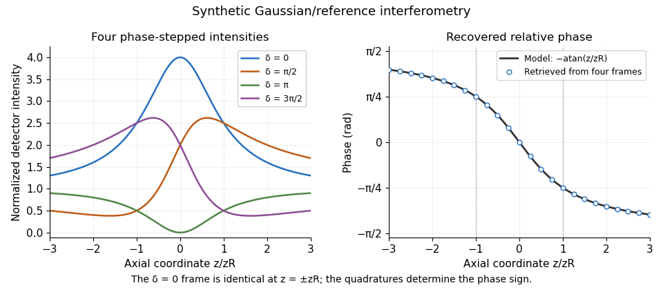
Original synthetic four-step interferometry of a Gaussian beam: symmetric single-frame readings become distinguishable through phase quadratures. No experimental data are shown.
Details. Curvature bias in Gouy-phase measurements is important away from the axis: the signal adds to its spatial phase. Fit or remove that term when using multiple pixels, retain calibrated phase steps and account for drift between frames. The recovered phase combines all coherent optical-path contributions until those controls isolate the Gouy phase.
Glucuronate is the conjugate base of glucuronic acid, formed by losing the proton of its carboxyl group. In the usual D series, the free monomer has molecular formula , compared with for the neutral acid. A six-membered-ring example is D-glucopyranuronate, whose official chemical record includes both alpha and beta anomers.[ref]
Protonation and anomeric configuration answer different questions. Removing a carboxyl proton changes charge; selecting alpha rather than beta specifies the arrangement at the anomeric center. Neither operation is the carbon-5 epimerization that distinguishes the glucuronate and iduronate series.
The Henderson-Hasselbalch equation quantifies the acid–base distinction. In an ideal dilute solution, . At a pH two units above the relevant , the ratio is , giving an anionic fraction . This example uses an offset from the dissociation constant rather than assigning an unverified numerical value to it.
The capsular space is the fluid-receiving space within the glomerular capsule, between its outer wall and the visceral surface formed by podocytes. Glomerular filtration delivers water and filterable solutes into this space, which is continuous with the lumen of the proximal tubule. It belongs to the tubular-fluid pathway, rather than the lumen carrying blood through glomerular capillaries.[ref]
Anatomy and Physiology 2e by J. Gordon Betts and others. Section25.4: renal corpuscle and capsular space
A useful tracing exercise follows two routes through a renal corpuscle. Blood enters and leaves through vessels; filtered fluid crosses the glomerular filtration barrier, enters the capsular space and exits into the tubule. A section showing both routes does not show direct mixing of whole blood with the capsular contents.
The receiving hydrostatic pressure also opposes further filtration. If every other term in a simplified trans-barrier pressure model is fixed, raising receiving pressure by lowers net driving pressure by the same amount. This hypothetical subtraction explains why arterial pressure alone is insufficient. In 1971, direct glomerular and proximal-tubular pressure measurements in rats were combined to estimate the driving force for ultrafiltration.[ref]
The Dynamics of Glomerular Ultrafiltration in the Rat by Barry M. Brenner and others. Abstract: servo-null micropipette measurements and pressure difference; quantitative correction noted on publisher page
Tau-leaping accelerates the Gillespie algorithm by approximating reaction rates as constant over an interval , then drawing all reaction counts for that interval at once. At state , with reaction propensity functions and stoichiometric vectors , the explicit step isThe leap condition requires the propensities to change little during the interval. Unlike event-by-event exact simulation, this introduces an approximation error controlled through the choice of .[ref]
Approximate accelerated stochastic simulation of chemically reacting systems by Daniel T. Gillespie. Section III, Poisson tau-leap construction
For with rate , the approximate number converted is Poisson with mean . The exact number converted over the interval is instead binomial with parameters and . The two agree to first order for small , but the Poisson draw can exceed and produce a negative count. Smaller or adaptive leaps and modified sampling rules address this limitation; freezing the rate is not automatically safe at low copy number.
The Perron-Frobenius operator transports a density under a map. For a piecewise smooth expanding interval map , relative to Lebesgue measure,Each inverse branch contributes its incoming density times its length-contraction factor. A change of variables gives , proving that probability is transported correctly.
In a metric space , a geodesic ray is an isometric embedding :Every finite segment therefore minimizes length between its endpoints. In Riemannian geometry, this is a globally minimizing unit-speed geodesic defined for all nonnegative times. Some authors use “ray” more loosely for any half-infinite geodesic, so the minimizing convention matters.
In Euclidean space, is a geodesic ray whenever . On a unit round sphere, a unit-speed great circle continues indefinitely as a geodesic, but it is not a ray: after time it returns to its starting point. In fact, a bounded metric space cannot contain a geodesic ray, since its points would have to lie arbitrarily far from .
A generalized eigenvalue is a scalar for which has a nonzero solution . For a regular square pencil this is equivalent, at finite , to .
For and , the generalized eigenvalues are two and three. If is invertible, these are the eigenvalues of , although explicitly forming that inverse is not necessary to solve the problem. Singular can introduce an eigenvalue at infinity, while a singular pencil is a separate case. For symmetric and positive-definite symmetric , transforming with gives a symmetric ordinary eigenproblem and hence real eigenvalues.[ref]
Eigenvalues and Schur Forms in the LAPACK Users' Guide. Generalized eigenvalue definition and symmetric-definite versus singular cases
For a regular matrix pencil , an eigenvalue at infinity is represented by a homogeneous pair with and . The eigenvector relation then requires with .
For and , the first coordinate has finite eigenvalue one and the second has an infinite eigenvalue. More generally, if are and the pencil is regular, its infinite algebraic multiplicity is . A singular pencil, whose determinant is identically zero, requires a different structural analysis and cannot be treated as an ordinary list of finite and infinite eigenvalues.[ref]
Eigenvalues and Schur Forms in the LAPACK Users' Guide. Generalized nonsymmetric eigenproblems: homogeneous pairs and regular versus singular pencils
Gear sliding velocity is the relative tangential surface velocity at a tooth contact. It must distinguish the common point where the tooth surfaces touch from the two material points instantaneously occupying it. For an ideal fixed-axis external involute pair, relative normal velocity vanishes, but relative tangential velocity generally does not. It is zero at the gear pitch point and grows with distance from it along the gear line of action.[ref]
Elements of Metric Gear Technology by SDP-SI. §3.1, common base-circle tangent, line of action and pitch-circle geometry
Let be the pitch point, a contact point and a unit direction along the line of action. Use a common positive rotation axis for both signed angular velocities. The rigid-body velocity law givesSubtracting these expressions and using equal velocities at givesThe result is perpendicular to the common normal, as the contact constraint requires. External gears rotate in opposite directions, so the sliding-speed magnitude is , rather than their speed difference in magnitude.
For and , at the signed tangential sliding velocity is ; at it is . Both vanish at . Doubling both shaft speeds doubles gear sliding velocity at the same contact location, while leaving the ideal gear ratio unchanged. This connects geometry and running speed to gear sliding-friction loss. The formula concerns a two-dimensional spur gear contact; general three-dimensional contact requires the complete surface velocities and common normal.
Gear sliding-friction loss is the rate at which relative tooth-flank sliding dissipates mechanical energy. In a simple Coulomb friction model with normal contact load , coefficient of friction and gear sliding velocity , the nonnegative dissipated power isThis is a local contact model, rather than the entire gearbox loss. Manufacturer guidance distinguishes gear-meshing losses from losses in rotating supports and warns that overall gear efficiency depends on load and speed.[ref]
Technical Data Gearhead by Citizen Micro. “Gear Efficiency”, meshing/support losses and load- and speed-dependent efficiency
To derive the sign, let along the common tangent. The friction force on surface1 is and that on surface2 is . Their combined mechanical power is . The corresponding positive quantity is the rate of mechanical energy loss. At zero sliding the ideal Coulomb sliding-loss term vanishes, even though another resistance mechanism can remain.
For a fixed-axis external spur gear pair with , gives . Hypothetical and give . Holding these load and friction assumptions fixed while doubling both shaft speeds doubles the instantaneous loss at that geometric point.
Gear friction work per engagement integrates this varying loss through the active gear path of contact. If one pair carries a constant , the contact coordinate runs from to at constant speed , givingFor , and , the preceding loads and speeds give about . Real tooth pairs share varying loads; an overall loss calculation must sum the applicable contacts and integrate their actual loads, sliding and friction model.
A gear inspection common-region comparison evaluates repeated surface observations on the same registered portion of a tooth flank. It prevents a changed gear pitting inspection mask from being mistaken for a change in damage. The region must be common in surface coordinates, not merely occupy the same pixel positions in two camera images.
After image registration, let and be inspection-mask indicator functions on one reference grid. Their common mask isIf classifies pitting at time and is represented surface area, defineThe identical denominator makes the difference a comparison within the same eligible area. It does not eliminate errors in registration or image segmentation.
An original example has 10000 eligible equal-area pixels at the first inspection and 8000 at the second, with 7000 in common. In the common region, pitted counts rise from 140 to 210: fractions rise from to , a change of one percentage point or relative to the original fraction. Suppose total pitted counts were 200 and 240 across the separate full masks. Their raw difference, 40 pixels, is not the same quantity as the 70-pixel increase within the common region.
A gear inspection coverage audit should also record the excluded areas and why they disappeared or became newly visible. An intersection-only result can miss damage on an edge that the second camera view no longer captures. Keeping the original images makes that loss of coverage visible to a later reviewer.
Common inputs can correlate the two estimated fractions. In general,This is the usual correlated-input uncertainty propagation, not an assumption that neighboring image pixels are independent.[ref]
Evaluation of measurement data — Guide to the expression of uncertainty in measurement by JCGM. Section 5.2, covariance of correlated inputs
A primary NASA endurance study linked repeated physical inspections with vibration and debris observations; the common-region formalism specifies one way to make such repeated surface measurements comparable.[ref]Gear Fault Detection Effectiveness as Applied to Tooth Surface Pitting Fatigue Damage by David G. Lewicki and others. Printed pp. 2–5, test procedure, inspections and damage comparisons
The gear path of approach is the part of the active gear path of contact followed before the contact reaches the gear pitch point. For a conventional external involute pair in the stated driving direction, contact starts where the driven gear's tip circle intersects the usable gear line of action, and then moves toward the pitch point. This is a straight-line distance along the common normal, not an arc around a pitch circle.[ref]
KHK Gear Nomenclature. “Length of Path of Contact”, approach segment from first contact to the pitch point
Let gear1 drive gear2. Write for gear2's tip radius, for its base radius, for its operating radius and for operating pressure angle. A right triangle from the base-circle tangency gives tip-to-tangency distance . Subtracting the pitch-point-to-tangency distance givesThis formula assumes the full tip-limited interval is usable without interference or profile truncation.
For an original standard module2,20/40-tooth pair at60mm center distance and20degree reference angle, gear2 has tip radius42mm, operating radius40mm and base radius . Consequently . If gear1 rotates at , contact advances along the line at , giving an approach contribution to gear contact duration of about . This contact-location speed differs from gear sliding velocity, which tends to zero on arriving at the pitch point.
The total active length adds gear path of recess. Reversing the followed engagement direction exchanges which segment is called approach and which is recess. If altered usable flanks exclude the nominal pitch point, an assumed positive tip-limited formula must not replace an inspection of the actual active interval.
The gear path of recess is the part of the active gear path of contact followed after passing the gear pitch point, in the stated driving direction. For a standard external involute pair driven by gear1, contact ends at the driving gear's tip circle when that tip bounds the usable profile. The recess length lies on the gear line of action; it is not an arc of the gear pitch circle.[ref]
KHK Gear Nomenclature. “Length of Path of Contact”, recess segment from pitch point to final contact
Use driving-gear tip radius , base radius , operating radius and operating pressure angle . The base-circle tangent triangle givesFor a standard module2,20/40-tooth pair at60mm separation and20degree reference angle, , and yield . The corresponding gear path of approach is about5.0586mm, so the pitch point does not bisect the active contact interval.
At driving angular velocity , the contact-location speed is . Recess therefore lasts about4.891ms. Adding approach gives gear contact duration . Tooth-passage frequency is , so , agreeing with the transverse gear contact ratio calculated as active length divided by gear base pitch.
A shorter usable driving flank reduces recess and can change gear sliding-friction loss, because sliding grows with distance from the pitch point. The tip-circle formula alone cannot describe profile modifications or an interfering contact. The geometry and direction must be specified before applying the approach/recess labels.
Pinned article: Introduction to the OurBigBook Project
Welcome to the OurBigBook Project! Our goal is to create the perfect publishing platform for STEM subjects, and get university-level students to write the best free STEM tutorials ever.
Everyone is welcome to create an account and play with the site: ourbigbook.com/go/register. We belive that students themselves can write amazing tutorials, but teachers are welcome too. You can write about anything you want, it doesn't have to be STEM or even educational. Silly test content is very welcome and you won't be penalized in any way. Just keep it legal!
Intro to OurBigBook
. Source. We have two killer features:
- topics: topics group articles by different users with the same title, e.g. here is the topic for the "Fundamental Theorem of Calculus" ourbigbook.com/go/topic/fundamental-theorem-of-calculusArticles of different users are sorted by upvote within each article page. This feature is a bit like:
- a Wikipedia where each user can have their own version of each article
- a Q&A website like Stack Overflow, where multiple people can give their views on a given topic, and the best ones are sorted by upvote. Except you don't need to wait for someone to ask first, and any topic goes, no matter how narrow or broad
This feature makes it possible for readers to find better explanations of any topic created by other writers. And it allows writers to create an explanation in a place that readers might actually find it.
Figure 1. Screenshot of the "Derivative" topic page. View it live at: ourbigbook.com/go/topic/derivativeVideo 2. OurBigBook Web topics demo. Source. - local editing: you can store all your personal knowledge base content locally in a plaintext markup format that can be edited locally and published either:This way you can be sure that even if OurBigBook.com were to go down one day (which we have no plans to do as it is quite cheap to host!), your content will still be perfectly readable as a static site.
- to OurBigBook.com to get awesome multi-user features like topics and likes
- as HTML files to a static website, which you can host yourself for free on many external providers like GitHub Pages, and remain in full control

Figure 2. You can publish local OurBigBook lightweight markup files to either OurBigBook.com or as a static website.
Figure 3. Visual Studio Code extension installation.
Figure 5. . You can also edit articles on the Web editor without installing anything locally. Video 3. Edit locally and publish demo. Source. This shows editing OurBigBook Markup and publishing it using the Visual Studio Code extension. 
- Infinitely deep tables of contents:



All our software is open source and hosted at: github.com/ourbigbook/ourbigbook
Further documentation can be found at: docs.ourbigbook.com
Feel free to reach our to us for any help or suggestions: docs.ourbigbook.com/#contact