Topics (384k) Articles (398k) Users (410) Discussions (242) Comments (383) Files (13k) New article

A periodic orbit obstruction is a necessary compatibility condition for solving a cohomological equation. If an dynamical observable is a flow coboundary, , where differentiates along the flow, then on a periodic orbit of period ,A nonzero integral therefore rules out a single-valued transfer function . Under suitable transitive Anosov flow and Hölder regularity hypotheses, the Livšic theorem provides a converse. Without those dynamical and regularity assumptions, vanishing periodic integrals alone is not a general existence theorem.[ref]
Abelian Livšic theorems for Anosov flows by Richard Sharp. Introduction, classical periodic-orbit theorem and equation (1.1)
A ray floret is a flower whose corolla has a conspicuous extended, strap-like limb, typically projecting from the edge of an Asteraceae flower head. The apparent petal around a daisy-like head is therefore part of a whole floret. It is not a single petal belonging to one giant central flower. Depending on the species, ray florets may be female or sterile; their appearance alone does not establish fertility.[ref]
Asteraceae in the New South Wales Flora Online. Description: ray-corolla form and reproductive variation
Compare an intact head with a dissection: trace one outer ray to its own base, then inspect a central disc floret. The contrast is between two floral forms assembled into one inflorescence. Counting rays around the edge does not count the full complement of constituent flowers, because it misses the central units.
A disc floret is a small tubular flower within a flower head of Asteraceae. Its corolla usually ends in approximately equal lobes. In a radiating daisy-like head, disc florets occupy the central region, surrounded by ray florets; other heads can contain only tubular flowers. The word disc describes the collective arrangement, not a flat disc-shaped individual flower.[ref]
Asteraceae in the New South Wales Flora Online. Description: corolla forms and combinations within a head
A hand-lens comparison makes the unit clear. Lift one central disc floret from a common daisy head and follow its narrow corolla down toward the ovary. Then compare an outer ray floret with its extended strap-like corolla. Both are whole flowers, even though the outer one resembles a single petal of a larger blossom.
An illustrative count of twenty central disc florets and ten peripheral ray florets describes thirty constituent flowers, not thirty petals of one flower. Whether each unit is fertile must be checked from its reproductive structures and the species, rather than inferred just from its position.
Floating-pinion centering stiffness describes the local restoring-force response of the mounting to displacement along a specified balancing coordinate. If mounting reaction is , a convenient positive restoring convention isFor , has force-per-length units. A rotational coordinate would require a torque-per-angle stiffness instead; the coordinate and displacement endpoints must be stated before comparing values.
In an original symmetric model of a floating pinion, two compressed mesh reactions obeyWith support reaction , equilibrium givesThe rigid-centering imbalance is , soBoth reactions must remain nonnegative for this two-contact model to apply.
For , and , choose . Displacement is and reactions are and . Raising to reduces displacement to but gives forces and . Stronger centering keeps the location closer to its reference while preserving more of the original imbalance.
Dynamic response is another question. With an effective mass and viscous coefficient , the same linearized floating-pinion balancing mode obeysIts undamped natural frequency is in angular-frequency units. A favorable static split does not by itself establish favorable dynamic behavior, and the toy mode does not include every shaft or housing motion.
A stiffness measurement should separate mounting reaction from the mesh reactions or report the combined assembly stiffness explicitly. The primary 2002 face-gear program used a cantilevered mounting to permit pinion balancing and examined a constrained comparison; it did not establish one universal centering stiffness for all transmissions.[ref]
Development of Face Gear Technology for Industrial and Aerospace Power Transmission by Gregory F. Heath and others. Introduction, printed p. 1; Conclusions, printed p. 84, floating mounting and modified fixed-pinion comparison
Length-prefix validation before allocation checks that an encoded payload length is permitted and safely usable before requesting memory allocation based on it. A fixed-width length field bounds what the encoding can represent; an application can impose a smaller limit. TLS vectors, for example, have explicitly specified minimum and maximum byte lengths.[ref]
The Transport Layer Security Protocol Version 1.3 (RFC 8446). §3.4, variable-length vectors and permitted bounds
For an original decoder model, let be the decoded unsigned payload length, the application limit and the bytes remaining in a complete input buffer after the prefix. Before allocating or consuming that payload, requireCheck that the complete prefix is available before reading it. For a two-byte big-endian prefix
02 01, . With and , the input fails both checks. Prefix 01 2c instead declares bytes and satisfies these two bounds. The example counts only payload bytes in .Arithmetic needs its own bound. If an allocation includes additional bytes and the size type's maximum value is , verify and before forming . Computing the sum first can already cause integer overflow. Similarly, when allocating elements of positive size , check before multiplication.
For a streaming decoder, can mean that more input is needed rather than that the final message is malformed. It still does not justify consuming unavailable bytes or allocating beyond the stated resource limit. Nested fields need bounds relative to their enclosing field. These checks establish safe structural handling of a length-prefixed encoding; they do not authenticate the sender or validate the payload's meaning.
The critical fibre length is the minimum embedded fibre length needed to develop a specified tensile stress in a simple interfacial-load-transfer model. For diameter , fibre strength and constant limiting interfacial shear stress ,Each half of the fibre builds axial force from its end through interfacial shear; balancing that transferred force against the strength load gives the formula. It is a model-dependent criterion, not a universal length of the material. Nonuniform shear, imperfect bonding and fibre orientation modify actual composite behavior.
The dyadic adding machine is addition by one on the space of infinite binary digit sequences, interpreted with the least significant digit first. Carries propagate toward later digits: . The all-ones sequence maps to the all-zeros sequence.
Equivalently, it is the compatible collection of cyclic maps for all , or translation by one on the 2-adic integers. Every orbit visits every finite binary cylinder and is therefore dense. At the Feigenbaum attractor, this describes the order of visits to nested intervals; it is not the digit-discarding evolution of a full shift.
Drift rejection by contrast orthogonality removes specified additive time trends from a load comparison by choosing contrast weights orthogonal to those trends. In an aerodynamic interference experiment, it prevents an assumed form of balance-zero drift from being confused with nonadditivity between component configurations.
For observations at times , writeThe columns of specify nuisance trends and their unknown amplitudes. The drift contribution vanishes for every amplitude exactly whenFor polynomial instrumental drift through degree , the columns are , so the conditions are for . This orthogonality is a statement about actual observation times, not merely the number of repetitions.
An original eight-run construction uses equally spaced times in a fixed time unit and the configuration orderFor the factorial contrast for aerodynamic interference, chooseEach configuration occurs twice and its total weight is the coefficient required for . Direct summation givesThe schedule rejects constant, linear and quadratic additive drift, but a cubic term leaves bias . If equal run spacing changes, the moments must be recomputed. If independent residual errors have common variance , the contrast variance is ; correlated errors instead require the full covariance matrix.
Rejection must preserve the physical signal. If a desired signal column lies in the nuisance column space, every vector rejecting that space also rejects the signal. Orthogonal projection exposes this identifiability limit; collecting more readings in the same confounded arrangement need not fix it. Gain drift, configuration-dependent tare and abrupt offsets are also outside the stated additive polynomial model.
Kenneth E. Ward's original attached- and isolated-strut measurements motivate separating combined load from component drag.[ref]
Interference Effects and Drag of Struts on a Monoplane Wing by Kenneth E. Ward. Report abstract and Discussion of Results, interference versus isolated strut drag
The eight-run schedule here is a constructed design, not a reconstruction of that historical experiment.Window-capture sensitivity to mass offset describes how the extracted-ion window capture fraction changes when an ion peak shifts relative to a fixed extracted ion mass window. The shift is in the reported mass coordinate; it can change the selected signal even if the target's total peak area is constant.
For a normalized peak shape with offset and window boundaries , writeDifferentiation givesThe first-order response is determined by the signal density at the two boundaries. A symmetric peak centered in a symmetric window has equal boundary densities and hence zero first derivative. Zero first derivative does not mean perfect immunity: finite offsets can still reduce capture.
For an original Gaussian function model with standard deviation and half-width , let and be the standard normal density and standard normal cumulative distribution function. ThenFor small offsets the leading loss is consequently quadratic:With , the exact capture is 0.9545 at zero offset and 0.9270 at . The quadratic approximation gives 0.9275, close for this stipulated displacement. At the boundary , capture is about 0.5000 and a small-offset approximation is no longer appropriate.
An experimental check can re-extract the same recorded spectra with deliberately shifted windows while retaining the same time limits and extracted-ion chromatogram baseline. This isolates a software-selection effect. IUPAC's selected-mass profile definition supplies the measurement setting, rather than a claim that all instruments have Gaussian peaks.[ref] Wider windows may reduce target losses but admit interfering ions; mass resolving power and instrument calibration remain separate instrumental considerations.
An extracted-ion chromatogram baseline is a model of the signal underlying a selected chromatographic peak in an extracted ion chromatogram. Subtracting it helps assign an extracted-ion chromatogram peak area to the feature of interest. The baseline need not be zero or constant, and it is not automatically the signal from a separate reagent blank.
Let be the signal from an extracted ion mass window and let be the baseline over . The assigned extracted-ion chromatogram peak area isThe time-ordered mass selection follows the IUPAC extracted ion profile definition; the baseline is an additional integration-model choice.[ref]
Extracted ion profile in IUPAC Gold Book. Entry 12410, signal from selected mass-to-charge values across time-dependent spectra.
An original example takes and a baseline rising linearly from 1 to 3 signal units. Its integrated area is signal-unit minutes. If the recorded trace has total area 20, the corrected area is 12. Using a constant baseline 1 would subtract only 4 and assign area 16: a 33% overestimate relative to 12. No recorded ion signal changed; only its allocation between baseline and peak changed.
If a fitted baseline is over a duration starting at , then the subtracted area is . Chromatographic baseline-area uncertainty therefore includes the joint uncertainty of the fitted intercept and slope:This is a direct application of correlated-input uncertainty propagation.[ref]
Candidate baseline regions should be inspected for neighboring peaks, broad tails and drifting background. Two overlapping compounds can generate one smooth trace; subtracting a convenient baseline cannot establish chemical specificity. Record the integration boundaries, baseline model and treatment of negative corrected values. Those choices are necessary to interpret or reproduce a reported extracted-ion chromatogram peak area.
The worst-switching-phase settling bound for a first-order circuit maximizes the initial transient over the source's unknown switching wave phase. For the stable RC circuit, let its sinusoidal particular solution be , where , and let be the initial capacitor electric potential difference. The error identity in exponential settling bound for RC sinusoidal turn-on givesSince ranges from minus one to one,For a validated initial bound , the sharp uniform bound is therefore . It is attained by choosing the extreme initial value and the opposite steady-state wave phase. A normalized error tolerance is guaranteed thereafter ifThere is no division by the instantaneous sinusoid, so its zero crossings cause no singular relative-error specification.
For an original example, choose , , , and . The worst-case settling time is . Assuming an uncharged capacitor instead would give . That shorter guarantee requires the additional initial-state information.
A phase-locked test can measure a smaller mismatch, even zero for a specially matched initial condition, without contradicting the worst-case result. A valid comparison records both the switching wave phase and the capacitor's initial state. The MIT laboratory's square-wave natural-decay observation and sinusoidal amplitude/wave phase measurement provide the two underlying bench measurements.[ref]
Laboratory 11: Sinusoidal Steady State Response of RC and RL Circuits by MIT OpenCourseWare. Printed pp. 1–2
The result assumes the same linear first-order model throughout switching; additional modes or a time-varying component require another transient bound.Emission-spectrum mismatch in nail fluorescence subtraction is the error caused by correcting a detector reading with an assumed fluorescence spectrum that differs from the actual emitted spectral shape. Knowing total fluorescent power does not generally determine fluorescent detector current, because the detector/filter response varies with wavelength.
Let be the true normalized emission spectrum, the assumed normalized spectrum and the product of spectral responsivity and optical filter transmission. DefineFor a current , subtraction of givesAlthough , the response-weighted integral need not vanish. Equal total emitted powers can therefore require different corrections.
An original two-band example makes the effect visible. Suppose the effective responsivity is and in two nonoverlapping bands. If fraction of fluorescent power lies in the first band, . The assumed fraction gives , whereas the true gives . At and transmitted-band responsivity , the transmitted-power estimate is biased by . A true would be reported as after that excessive subtraction.
These are stipulated spectral shapes and coefficients, not measured nail spectra. If were constant over the entire emission band, normalization would make this particular shape error vanish. A selective system generally sacrifices that invariance to distinguish transmitted excitation light from emission. Responsivity characterization and spectral measurement must therefore accompany a proposed subtraction.
The primary nail experiment explicitly included a correction for fluorescence while measuring transmission with a monochromator, integrating sphere and photodiode.[ref]
The transmission of optical radiation through human nails by S. G. Parker and B. L. Diffey. Abstract, fluorescence correction and apparatus
That observation motivates the distinction between emitted power and detected current; it does not specify the two-band correction model above. Fixing an assumed spectrum in software does not establish that the specimen actually has that spectrum.A call spread combines a long European call option of strike with a short European call of higher strike , on the same underlying financial asset and expiry. Its terminal financial payoff isThe higher-strike call cancels the growth beyond , leaving a capped increasing payoff. The opposite long/short convention negates this payoff.
For strikes and , terminal prices give payoffs . These are payoff calculations before accounting for the initial price of the position. Dividing by gives a continuous ramp between zero and one, which approaches the indicator of as the upper strike decreases to the lower one, away from the strike itself. This makes call spreads useful mathematical building blocks for approximating digital payoffs.
For a connected finite CW complex , choose a point in each open cell . An Euler chain is a singular chain of degree one withIt exists exactly when the Euler characteristic of is zero. Necessity follows because the total coefficient sum of every one-chain boundary is zero, whereas the displayed zero-chain has coefficient sum .
For sufficiency, choose a base point and paths from to . Then has boundary equal to the required sum minus , so it works when . Connected CW complexes are path connected, which justifies choosing these paths.
With the cell points fixed, two Euler chains differ by a cycle and define the same Euler structure when that cycle is a boundary. Adding homology classes makes Euler structures a torsor for . This extra choice removes an ambiguity in Turaev torsion.[ref]
Surgery formula for torsions and Seiberg-Witten invariants of 3-manifolds by Vladimir Turaev. Section4.1, Euler-chain definition and free transitive homology action, printed p14
A simply supported beam is prevented from moving transversely at its two supports while its ends remain free to rotate. In the small-deflection Euler-Bernoulli beam equation, a uniform span with transverse displacement and positive beam flexural rigidity has the support boundary conditionsHere is Young's modulus and is the second moment of area about the bending axis. The second pair expresses zero applied endpoint bending moment, since in the convention used here. It does not set the endpoint beam cross-section rotation or slope to 0. A clamped boundary condition instead constrains both displacement and slope.
For an original derivation, apply a downward central point force and take positive downward. Assume small elastic deflections, constant and no axial preload. Symmetry and force balance give an upward reaction at each support. On the left half, the bending moment is , so . Integrate twice, using and the symmetry condition , to obtainThus the midspan compliance of a simply supported beam isThe endpoint slopes are and : they are generally nonzero. This support geometry and central-load formula are used to infer material stiffness from a three-point bending test.[ref]
The moment-free natural boundary condition for a beam also follows from the principle of virtual work. For a central load, the total potential energy is . An admissible virtual displacement satisfies , while its endpoint first derivatives remain free. Two integrations by parts produce the boundary contributionThe terms multiplying vanish because the endpoint displacements are prescribed. Arbitrary endpoint values of then require there. The free end rotation and zero end moment are conjugate parts of the same variational boundary condition.
Clamping both ends changes the central-load deflection to , one quarter of the simply supported value for the same . It introduces endpoint reaction moments; it does not merely rename the same support. The clamped-beam Green function provides the corresponding fourth-order boundary-value solution. The support conditions likewise determine the simply supported beam normal modes, so a static stiffness measurement and a vibration measurement must use the same mechanical support model when they are compared.
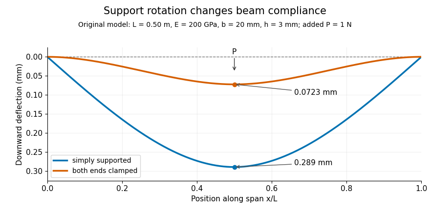
Original central-load beam profiles: allowing support rotation gives four times the midspan deflection of clamping both ends.
Details. A three-point bending test places a specimen on two separated supports and applies a central force. A load cell measures force, and a midspan displacement readout measures response. A direct plunger and extensometer can measure specimen deflection separately from machine crosshead displacement, as in the published Instron fixture arrangement.[ref]
Three Point Bend Test Fixtures by Instron. Principle of Operation and midspan deflectometer description
Fitting a proportional small-load segment estimates , where is the measured incremental midspan compliance. Record support spacing, load position and cross-section dimensions with that estimate.For stipulated , rectangular width , thickness and , the second moment of area is and . An incremental central load gives incremental deflection under the simply supported model, versus for the clamped model. Incremental readings remove an unchanged baseline deflection in this linear model; support settling, contact indentation and large rotations require separate interpretation.
Beam flexural rigidity is the coefficient relating a slender beam's bending moment to its curvature in linear bending. For a homogeneous material with uniform Young's modulus over the material area,where is distance from the appropriate neutral axis. The magnitude relation is ; signs depend on the chosen moment and curvature conventions. Integrating the linear bending stress over the section gives this coefficient.[ref]
For an original rectangular example, choose width , bending thickness and . The second moment of area is , giving . Doubling only the thickness multiplies by eight. Rotating the original rectangle by ninety degrees about its length instead exchanges width and thickness: increases by even though material area and modulus are unchanged.
Thus a bending experiment measures a combination of material response and geometry. Extracting requires the correct bending axis and second moment of area; the three-point flexural test is one route. This beam coefficient has units , distinct from the plate coefficient called bending stiffness. If modulus varies across a section, the relevant stiffness requires a material-weighted area integral and the appropriate neutral axis, rather than an arbitrary average modulus multiplied by .
Beam cross-section rotation is the signed change in orientation of a material section in the bending plane. The Euler-Bernoulli beam equation assumes that sections remain plane and perpendicular to the deformed centreline. With a consistent angle convention, the section rotation therefore agrees with the centreline tangent angle; for a graph ,The last step is a small-angle approximation, with the angle measured in radians. This kinematic relation underlies the axial bending strain, rather than being an extra condition imposed by every support.[ref]
For an original geometric profile, take with . At , the slope is , while the exact tangent angle is radians. Replacing it by overestimates the angle by about 0.33 percent. This is a chosen shape illustrating the approximation, not a measured equilibrium profile.
The beam shear angle records a possible difference between centreline slope and section rotation in a model that permits transverse shear strain. The Euler-Bernoulli kinematics set that difference to zero; a short or shear-compliant specimen can require a different model. A simply supported beam leaves its end section rotation free, whereas a clamped boundary condition prescribes it. Neither zero transverse displacement alone nor zero endpoint bending moment requires zero rotation.
A rotational spring boundary condition for a beam lets an endpoint rotate while imposing a restoring torque proportional to that rotation relative to its support. Let be the spring stiffness, with zero rest angle. Its stored elastic energy is , where the small beam cross-section rotation is .
At a right endpoint whose transverse position is fixed, add this energy and the applied-couple potential to the bending energy. The coefficient of the free rotation variation isHere is beam flexural rigidity, and is defined by external virtual work . End moment and rotation are conjugate variables in the beam principle of virtual work.[ref]
The Concept of Stress, Generalized Stresses and Equilibrium by Tomasz Wierzbicki. §§3.4–3.5, equations3.46 and3.52–3.57
The spring term and the following example are independently derived. At the left endpoint, the bending boundary term has the opposite sign: with no applied end couple, .For an original fixture model, hold the left endpoint position fixed, restrain its rotation by the spring, and apply a downward end force at distance . The root moment magnitude is , giving root rotation . Bending relative to that rotated root contributes to the tip displacement; rigid root rotation contributes . ThusWith , , and , these contributions are and , giving total. Root rotation is radian, within the stipulated small-rotation model.
As increases without bound, the root approaches a clamped boundary condition. At zero stiffness this particular end-loaded arrangement becomes a rotational mechanism; it has no finite static deflection for nonzero . A small-couple fixture check can estimate from measured moment and angle. The resulting beam root rotational compliance is distinct from deformation of the beam material.
An esophageal balloon catheter is the tube-and-balloon instrument used to transmit a pressure signal from a balloon in the oesophagus to a pressure sensor. The esophageal balloon is the coupling element; the catheter also introduces a gas-filled line, connections and an external measurement chain. Those components can affect both baseline pressure and dynamic response.
The physiological filling study by Francesco Mojoli and collaborators shows why treating the assembly as an ideal pressure wire is inadequate: changing balloon filling altered pressure-change transmission and wall-related baseline pressure.[ref]
In vivo calibration of esophageal pressure in the mechanically ventilated patient makes measurements reliable by Francesco Mojoli and others. Abstract, Methods and Results
This establishes a measurement dependence, not one universal filling volume for every catheter and surrounding pressure.A minimal model of pneumatic response lag of an esophageal catheter iswhere is a varying source pressure and the sensor output. For a step from to , the response isWith a stipulated , 63.2 percent of the step appears after 0.10 s and 95.0 percent after 0.30 s. These are model calculations, not specifications of a clinical device.
This dynamic error differs from a fixed offset: waiting longer removes the modeled step-response lag but not a baseline bias. A comparison against a known pressure waveform can test the instrument's response, while an esophageal balloon occlusion test addresses transmission in the measurement setting. Neither validation alone proves that esophageal pressure equals regional pleural pressure throughout the lung.
Pinned article: Introduction to the OurBigBook Project
Welcome to the OurBigBook Project! Our goal is to create the perfect publishing platform for STEM subjects, and get university-level students to write the best free STEM tutorials ever.
Everyone is welcome to create an account and play with the site: ourbigbook.com/go/register. We belive that students themselves can write amazing tutorials, but teachers are welcome too. You can write about anything you want, it doesn't have to be STEM or even educational. Silly test content is very welcome and you won't be penalized in any way. Just keep it legal!
Intro to OurBigBook
. Source. We have two killer features:
- topics: topics group articles by different users with the same title, e.g. here is the topic for the "Fundamental Theorem of Calculus" ourbigbook.com/go/topic/fundamental-theorem-of-calculusArticles of different users are sorted by upvote within each article page. This feature is a bit like:
- a Wikipedia where each user can have their own version of each article
- a Q&A website like Stack Overflow, where multiple people can give their views on a given topic, and the best ones are sorted by upvote. Except you don't need to wait for someone to ask first, and any topic goes, no matter how narrow or broad
This feature makes it possible for readers to find better explanations of any topic created by other writers. And it allows writers to create an explanation in a place that readers might actually find it.
Figure 1. Screenshot of the "Derivative" topic page. View it live at: ourbigbook.com/go/topic/derivativeVideo 2. OurBigBook Web topics demo. Source. - local editing: you can store all your personal knowledge base content locally in a plaintext markup format that can be edited locally and published either:This way you can be sure that even if OurBigBook.com were to go down one day (which we have no plans to do as it is quite cheap to host!), your content will still be perfectly readable as a static site.
- to OurBigBook.com to get awesome multi-user features like topics and likes
- as HTML files to a static website, which you can host yourself for free on many external providers like GitHub Pages, and remain in full control

Figure 2. You can publish local OurBigBook lightweight markup files to either OurBigBook.com or as a static website.
Figure 3. Visual Studio Code extension installation.
Figure 5. . You can also edit articles on the Web editor without installing anything locally. Video 3. Edit locally and publish demo. Source. This shows editing OurBigBook Markup and publishing it using the Visual Studio Code extension. 
- Infinitely deep tables of contents:



All our software is open source and hosted at: github.com/ourbigbook/ourbigbook
Further documentation can be found at: docs.ourbigbook.com
Feel free to reach our to us for any help or suggestions: docs.ourbigbook.com/#contact