Topics (384k) Articles (398k) Users (410) Discussions (242) Comments (383) Files (13k) New article

Gear contact duration is the time for a specified tooth pair to traverse its active gear path of contact. For a fixed-axis external spur gear pair at constant speed, the contact location advances along the gear line of action at the common gear base-roll speedThis is the speed of the contact location along a geometric line, not the relative tooth-surface gear sliding velocity. The latter vanishes at the gear pitch point, while the contact location continues moving. For active path length , duration is . The geometry relates gear contact ratio to active path length divided by gear base pitch.[ref]
The time between successive tooth-pair entries is , with gear mesh frequency . Since for compatible operating geometry, the base-circle distance advanced per entry isConsequentlyA contact ratio above1 means one pair remains engaged after the next pair enters; it does not mean one pair contacts for an entire shaft revolution.
For the standard module2,20/40-tooth example with20degree reference angle, active length is9.65457mm and base pitch is5.90426mm. At driving angular velocity , , and . The entry interval is6.28319ms, giving . Doubling both shaft speeds halves duration while preserving geometric gear contact ratio. Variable speed requires integrating the changing base-roll speed; a helical gear also needs a stated transverse slice or a whole-face contact convention.
The gear contact-stress load factor is the multiplier associated with the face-load term in a contact-stress calculation where Hertzian contact pressure scales with the square root of local line load. It distinguishes a stress ratio from the underlying gear face load factor. The historical definition of compares maximum line-load intensity with the mean over the evaluation width.[ref]
For ideal elastic line contact, hold the effective geometry and material fixed. Write the peak pressure aswhere is load per contact length, the effective elastic modulus and the effective radius. If the largest line load is , division by the pressure calculated from the mean line load givesThe square root follows from the pressure model; it is not a second independent multiplier on the load.
For an original example, a face-load ratio gives a stress multiplier . A mean-line-load reference pressure would become under these assumptions. Multiplying pressure directly by would instead give and count the load ratio as though it were a stress ratio. Increasing effective line load fourfold doubles this model pressure.
Small relative uncertainties also scale differently:Thus a small relative change in produces about a relative change in its square root to first order. This sensitivity concerns that term alone; uncertainties in material, geometry and the reference load remain.
A local stress scaling does not predict gear surface pitting life on its own. Contact position, curvature, load history and material response matter. A primary NASA analysis explicitly combined varying tooth loads and contact geometry with a fatigue-life model.[ref]
Predicted Effect of Dynamic Load on Pitting Fatigue Life for Low-Contact-Ratio Spur Gears by David G. Lewicki. Summary, printed p. 1; Analysis, tooth-contact intervals and varying curvature/load
A real rating must keep all factors and load conventions consistent with the chosen method.A gear contact marking test makes a gear contact pattern visible by using a thin contrasting marking layer and rolling the mating gears under stated conditions. The observed transfer or removal of the layer locates the region where the flanks meet closely enough to mark. A useful test record includes the marked flank, rotation direction, mounting position, backlash and applied torque. Manufacturer guidance discusses tooth-surface contact as an assembly and alignment check.[ref]
A controlled comparison changes one alignment setting while keeping the same marking method and loading condition. A shift of the mark toward an edge then records a change in the mesh geometry. Changing layer thickness at the same time would confound that comparison: the visible pattern is the response of the surfaces and the marking process together.
An original threshold model illustrates this limitation without claiming a universal paint law. Suppose an unloaded gap over a face isStipulate that a mark appears wherever , with gear marking-layer gap threshold . At the marked width is ; at it is . The indicated coverage doubles even though the underlying gap is unchanged. Real transfer also depends on deformation and the marking material.
Nor does a broad mark uniquely determine the gear face load distribution. Operating torque deforms teeth, shafts and supports, so a lightly loaded pattern can differ from a loaded one. The historical gear-rating standard distinguishes comprehensive loaded assessment from the limited information in a bearing pattern.[ref]
A meaningful validation pairs the pattern with an independent load-sensitive observation, such as tooth-root strain, or a checked deformation model. The question is whether the setup places contact where intended under the specified condition, rather than whether one visually attractive mark proves uniform pressure at every operating load.
For an isolated Gaussian pulse, the relation between laser pulse energy and peak power depends on the pulse-width convention. Here is the total incident radiant power, the background is zero, and denotes the power full width at half maximum. Integrating over the entire pulse defines its positive energy .
Pulse energy, peak power and average power resolve different information. Consider a Gaussian pulse withThe chosen pulse duration is the full width at half maximum of radiant power: . It refers to radiant power, rather than the wave amplitude of the electric field. The Gaussian integral gives the relation between Gaussian pulse energy and peak power:The pulse energy shape factor is . It equals for this power profile; a rectangular pulse of duration has . Knowing only a width and an integrated energy therefore requires a pulse-shape assumption before inferring peak power.
An equivalent form makes the normalization transparent. Write the pulse centre as , and let denote the standard deviation of its energy-normalized pulse profile:The ratio is a probability density function in the mathematical sense: it is nonnegative, has units , and integrates to one. Here it weights the pulse's energy over time. Its normal distribution profile has mean and variance . This gives without a separate area estimate.
For a stipulated and , the power full width at half maximum is and the peak power is . Confusing the standard deviation with the full width at half maximum would insert the wrong duration into the conversion.
The Gaussian pulse field-envelope width is a second distinct convention. If a fixed spatial field profile gives for a constant , the wave amplitude envelope obeysConsequently its amplitude full width at half maximum is . Inserting into the formula for a power-width input underestimates the true peak power by a factor . State which measured waveform defines the width.
An electrical photodetector trace can also be broadened by its impulse response. The optical pulse-width inference therefore needs a characterized detector response.[ref]
The Gaussian pulse time-gate energy fraction is the share of an isolated pulse's laser pulse energy admitted by a finite time window. The result below acts on incident optical radiant power. Let be the power full width at half maximum, and first place the pulse centre and the detection time gate centre at zero.
A detection time gate need not collect the whole pulse. Integrating the same profile only over gives the Gaussian pulse time-gate energy fractionwhere is the error function. A gate as wide as the power full width at half maximum collects only , or 76.10% of the pulse energy. The pulse has nonzero Gaussian tails outside that interval. A real readout's impulse response can extend the required integration window further.
Alignment adds a parameter. Let the pulse centre be , the gate centre be , and write the Gaussian gate centring error as . Put . Integrating the normalized Gaussian pulse profile over the gate givesAt the two error function terms reduce to the centred formula above. With and , the captured fraction drops to . The pulse centre then lies on a gate edge. Merely keeping the gate width fixed does not keep its collected energy fixed.
The gate works best when centred. With the centred energy-normalized pulse profile and , differentiation of givesA Gaussian function is an even function about its centre and decreases with distance from that centre. Thus for , and symmetry gives the opposite sign for . The same argument proves that a centred interval maximizes mass for an even unimodal density; unimodality supplies the required monotonicity.
A centred gate of width captures of the energy. Solving gives for 99% capture in this ideal model. The requirement changes if the centring error is nonzero.
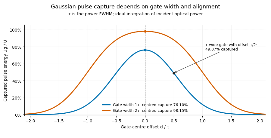
Pulse timing jitter can therefore create variation in gated energy even when every full pulse has the same . A wider gate reduces this loss but also changes admitted background and the chance of including neighbouring pulses. Measure the timing and detector response associated with the chosen gate.
For a detector modeled as a linear time-invariant system, its recorded waveform is a convolution of the optical input with its impulse response. NIST tested avalanche photodiode radiometers with roughly optical pulses, recorded their responses with an oscilloscope, and convolved measured responses with longer Gaussian inputs to estimate corrections. The detector and amplifier were characterized together.[ref]
Calibration Service for Low-level Pulsed-Laser Radiometers at 1.06 µm: Pulse Energy and Peak Power by Rodney W. Leonhardt. §§6.1–6.2, printed pp. 13–15: short-pulse excitation, sampling readout and numerical convolution
A gate applied to that electrical waveform must use the readout model rather than assuming the optical fraction is unchanged.The Gaussian pulse field-envelope width is the full width at half maximum of the magnitude of a Gaussian electric-field envelope. It differs from the FWHM of radiant power. For a fixed spatial mode with and constant ,The Gaussian pulse energy and peak power article derives this relation. Power-FWHM is also the convention explicitly used for PULSELENGTH in the primary source documentation.[ref]
Plane wave and beam source - Simulation object in Ansys Optics documentation. Standard source, PULSELENGTH definition and manual time-signal calculation
For an original example, a power width of corresponds to field-envelope width . At the field-envelope half-maximum points, the power is one quarter of its peak, since . At the power half-maximum points, the field magnitude is instead of its peak. A threshold applied to one measured quantity therefore does not define the other quantity's FWHM.
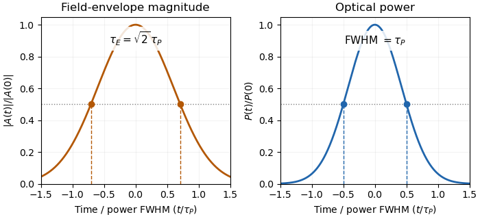
Squaring a Gaussian field envelope narrows its full width at half maximum by a factor of square root two.
Details. The envelope magnitude is distinct from the rapidly oscillating signed electric field. A direct photodetector generally supplies a power-related electrical trace, further modified by its impulse response; it is not a direct recording of the optical carrier's field envelope. Inserting an amplitude width into a power-width peak power formula consequently uses the wrong convention. State the observable and the response model with the reported pulse duration.
Waist-size mismatch in optical heterodyne mode matching reduces interference even when the beam centres coincide. For two circular Gaussian fields with matching polarization and wavefront curvature, define their radius ratio . The centred overlap from Gaussian beam overlap under lateral displacement givesHere is the beat-power fraction relative to a fully matched receiver at the same collected arm powers. Matching total power alone does not set .
An original tolerance calculation asks for . Solving the quadratic inequality givesThe allowed ratio is approximately to . With one radius , the other must be about – in this model. A radius gives only about beat power.
The interval has reciprocal endpoints because replacing by leaves the overlap unchanged. This reciprocal size-ratio ambiguity in centred Gaussian overlap means the beat magnitude alone cannot tell which beam is wider. Independent beam profiling or a known reference radius resolves that ambiguity.
NIST's heterodyne metrology setup used single-mode fibre and polarization matching to establish a calculable modulation rather than infer matching from collected power alone.[ref]
Frequency response metrology for high-speed optical receivers by Paul D. Hale and others. PDF p. 1, Heterodyne measurements
The radius test above omits displacement, curvature mismatch, clipping and angular misalignment. Radii must be compared at the same receiving plane; equal spot sizes there do not by themselves establish the same full Gaussian optical mode.A galactic wind is a large-scale flow carrying gas, energy and momentum away from a galaxy. Stellar winds and supernovae can maintain a hot, pressurized component that expands out of a star-forming region; an active galactic nucleus can supply another driving mechanism. Cooler entrained gas can coexist with the hot component.
Observations must distinguish the wind from unrelated point sources and foreground emission. In M82, ROSAT measurements separated extended soft X-ray emission from compact sources and traced emission away from the galactic plane. The emitting gas need not be the freely expanding wind itself: shocked clouds can dominate the detected radiation.[ref]
ROSAT Observations of the Galactic Wind in M82 by Dave Strickland and others. Abstract, spatial separation and comparison of free-wind and shocked-cloud emission
A voltage gain determines a power gain only when the electrical conditions at both ports are included. The familiar equality between and requires a particular impedance relation; it is not a conversion between arbitrary voltage and power ratios.
Use phasors whose moduli are root mean square amplitudes, at one sinusoidal frequency. At a load with electrical impedance and electrical admittance , the current is . Its complex electrical power is , with the complex conjugate arising from the relative phase of the two sinusoids. Averaging over a cycle gives the active powerTo see the averaging step, write and similarly for . The product's cycle average is , the real part of . Peak-amplitude phasors instead require an extra factor .
Let describe the actual input impedance and the actual load impedance. Take and with nonzero terminal signals, and define currents into the amplifier at the input and into the load at the output. With the measured loaded voltage gain ,Thus requires equality of the relevant electrical conductances, not merely equality of impedance moduli. For example, input and load both have modulus , but their electrical admittances have real parts and . The multiplier is , so .
For real resistive ports this becomesTake an original example with measured , and . The voltage gain is , while the power gain is , or . An active buffer can reduce the signal's electric potential difference while delivering more signal power than it accepts at its input; the supply provides the additional energy.
The amplifier's output impedance is distinct from the connected load impedance. To show why that distinction matters, model its output by a Thévenin equivalent with open-circuit voltage and series resistance . The voltage divider givesWith and , the load produces the preceding example. Differentiating gives , so delivered power is largest at , as in the maximum power transfer theorem. Here its power gain is . Increasing much further makes approach but reduces delivered power. That high-load-impedance regime is impedance bridging, useful for sensing the source's voltage with little loading.
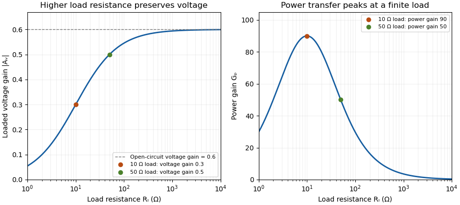
A bench demonstration uses a function generator, a known termination and an oscilloscope. The Keysight guide explains that an expected-load setting changes how amplitude is displayed for generators with a fixed series output impedance; a high-impedance load can receive twice the voltage expected for a matched termination.[ref]
Output Load Termination in the Keysight BenchVue Function Generator documentation. Output Load Termination, fixed output impedance and the 50-ohm/open-circuit examples
As an independent low-frequency resistive calculation, an open-circuit source of root mean square with series resistance delivers and to . Into it delivers about but only . The larger terminal reading accompanies much less delivered power. Specify the actual load, frequency and amplitude convention when comparing gain measurements.A dehiscence zone is a specialized region of a fruit where opening occurs during fruit dehiscence. Its organized cells form a reproducible release site in the pericarp. Differentiation of a separation layer and reinforcement of neighbouring tissue can cooperate to let the enclosing wall open in a controlled pattern.
In Arabidopsis thaliana, experiments with the SHATTERPROOF genes connected dehiscence zone formation and adjacent lignin deposition to SHATTERPROOF1 and SHATTERPROOF2. Disrupting both genes exposed a defect absent from the individual mutants.[ref]
SHATTERPROOF MADS-box genes control seed dispersal in Arabidopsis by Sarah J. Liljegren and others. Abstract; dehiscence-zone differentiation, lignification and single/double mutants
To distinguish specification from accidental rupture, compare the opening location and local cell anatomy across normal and altered fruits. A tear in a damaged pericarp can release seeds without demonstrating that a normal dehiscence zone formed. The useful mechanistic question is how local tissue identity makes one region a reliable opening site.
Xenopus is a taxonomic genus of African clawed frogs used in experimental biology. Xenopus laevis is an important example. Its large egg cells and oocytes make manipulations of individual cells possible, allowing researchers to change a defined component and observe development or membrane function.
In John Gurdon's 1962 somatic cell nuclear transfer experiments, nuclei from intestinal epithelium of feeding tadpoles were introduced into eggs whose own nuclear contribution had been removed. A nuclear marker helped identify the donor origin, while embryonic-nucleus controls tested whether the recipient eggs and procedure could support development. Successful development showed that differentiation did not necessarily eliminate the nuclear information needed for other cell types.[ref]
The Developmental Capacity of Nuclei taken from Intestinal Epithelium Cells of Feeding Tadpoles by J. B. Gurdon. Materials and Methods, nuclear marker and embryonic controls; Normal tadpoles
A different use treats the oocyte as a test cell for a cloned membrane protein. The 1993 aquaporin-2 study introduced the channel's RNA into Xenopus oocytes and measured the resulting increase in water permeability. Comparing injected and control cells turns swelling in a defined external solution into evidence that a candidate protein can provide a pathway for water across a cell membrane.[ref]
The osculating plane of a regular space curve at a point of nonzero curvature is the affine plane through the curve point spanned by its unit tangent vector and principal normal vector . Its normal is the binormal vector , so the plane is described byEquivalently, any regular parameter gives the span of and when these vectors are linearly independent. The second-order Taylor expansion then lies in this plane, which explains the name: it captures the curve's instantaneous bending.
A planar circle has its own containing plane as its osculating plane everywhere. For the helix at , the point is and a normal is , giving . At zero curvature the ordinary Frenet frame does not define a unique osculating plane.
Fluorescence fluctuation spectroscopy infers molecular properties from variations in detected fluorescence, rather than only from its time-averaged intensity. Diffusion of fluorescent molecules through a small illuminated region changes their number in that region; binding or changes of fluorescent state can change their brightness. Fluorescence correlation spectroscopy studies the time dependence of these fluctuations through an autocorrelation function.[ref]
For a stationary recorded intensity , put . A common normalized convention isFor an ideal uniformly weighted observation volume with independent equally bright particles, a Poisson distribution for the particle number gives , excluding the detector's instantaneous shot-noise contribution. The same mean signal could therefore arise from many dim particles or fewer bright ones, while their relative fluctuations differ. Real confocal profiles introduce an effective observation volume and model-dependent shape factors.
A confocal implementation uses a focused laser, spatial filtering of collected fluorescence and photon-sensitive detection to record an intensity trace. Faster diffusion usually shortens the correlation time. Binding kinetics, background, bleaching and detector effects can also modify the trace, so a fitted timescale needs a physical model.[ref]
Fluorescence Correlation Spectroscopy by the MIT So Lab. Detection-volume geometry, intensity fluctuations and limitations
The 1972 experiment by Douglas Magde and colleagues measured equilibrium fluctuations during binding of ethidium bromide to DNA. The measured correlations revealed both diffusion coefficients and chemical rate constants. It showed how apparently unwanted fluctuations can expose molecular dynamics without imposing a macroscopic concentration jump.[ref]
Thermodynamic Fluctuations in a Reacting System—Measurement by Fluorescence Correlation Spectroscopy by Douglas Magde and others. Abstract, equilibrium reaction-product fluorescence and DNA-binding experiment
A fluorometer measures fluorescence emitted by a sample under specified excitation and collection conditions. A spectral instrument can vary the excitation or observation wavelength; a simpler instrument can select fixed bands with filters. The reading depends on both the sample and the instrument, so converting an intensity into concentration requires an appropriate fluorescence calibration curve.
A typical spectrofluorometer sends source light through an excitation monochromator, illuminates the sample, then selects an emission band before a photodetector. Collection at to the incident beam reduces direct transmitted excitation reaching the detector. JASCO's illustrated configuration also sends a reference beam to a separate detector; dividing the fluorescence reading by the reference reading helps compensate for source fluctuations. These optical choices separate useful emission from excitation and stabilize its measurement.[ref]
Principles of fluorescence spectroscopy (3) - Instrument configuration by JASCO. Optical system and Fig. 7, excitation monochromator, right-angle fluorescence detection and reference-beam ratio
For an illustrative wavelength-selection example, hold the excitation band near and scan the observation band across longer wavelengths to record an emission spectrum. Holding the observation band near a selected emission peak while varying excitation instead records an excitation spectrum. The numbers specify a hypothetical setting, not a measurement of an identified dye. Slit widths select finite bands, so a nominal setting does not mean a single exact wavelength.
For quantitative work, measure a fluorescence blank containing the solvent and other background-contributing materials without the target fluorescent substance, then measure standards and unknowns with matching settings. Check detector saturation, source drift and repeatability before interpreting differences as changes of concentration. Changes in optical absorption, fluorescence quenching or photobleaching can change the response even when the intended concentration comparison is unchanged. A fluorometer measures an optical signal; a calibrated model supplies the inference about the sample.
An inner filter effect changes a measured fluorescence signal because light is absorbed within the sample along its excitation or detection path. In a primary inner filter effect, attenuation reduces excitation reaching the observed region. In a secondary inner filter effect, emitted photons are absorbed before reaching the detector. Both can distort intensity and spectral shape without requiring a change in the emitter's intrinsic fluorescence quantum yield.[ref]
Automatic Correction of Fluorescence Spectra for Primary and Secondary Inner-filter Effects (IFE) with Duetta by HORIBA. PDF p.1, Introduction and Fig. 1, excitation attenuation and emission reabsorption
A deliberately simplified geometry makes the effect quantitative. Consider a square sample cell viewed at , collecting from a small region at its centre. Let and be full-cell absorbances at the excitation and observed emission wavelengths. Each relevant path to or from the centre is half a cell width. Applying the Beer-Lambert law to those paths givesHere is the signal the same local emitters would give without attenuation along those paths. For stipulated values and ,The corresponding model correction multiplies the observed signal by about .
This is a centre-view approximation, not a universal correction for every fluorometer. A real detector collects from an extended region; geometry, scattering and strong absorption can invalidate the simple factors. The manufacturer's note describes measuring absorbance alongside fluorescence to support correction, rather than inferring attenuation from fluorescence intensity alone.[ref]
A useful diagnostic experiment measures a dilution series with unchanged settings and matched fluorescence blanks, recording both fluorescence and absorbance. Departure of signal per unit concentration from a constant suggests that the dilute linear model needs examination. Repeating with a shorter physical light path helps investigate optical attenuation. Dilution can also alter other sample properties, so this comparison does not by itself exclude fluorescence quenching, which changes emission through a different mechanism. Optical attenuation and quenching should not be treated as interchangeable explanations.[ref]
An excitation spectrum records a sample's fluorescence signal as the excitation wavelength is varied while the observation band is held fixed. It asks which incident wavelengths efficiently produce the selected emission. An emission spectrum instead varies the observed emission wavelength for a fixed excitation setting.
A fluorometer implements the scan with its excitation monochromator while keeping the emission selection fixed. For example, observing near while scanning excitation from to defines an illustrative excitation scan; it is not a measurement of a named substance. Finite band widths and the instrument's wavelength-dependent response are part of the measurement.[ref]
Principles of fluorescence spectroscopy (3) - Instrument configuration by JASCO. Optical system and Fig. 7, separate excitation and emission wavelength selection
[ref]Principles of fluorescence spectroscopy (4) - Notes on fluorescence measurements by JASCO. Spectral correction, instrument response versus sample spectrum
For a homogeneous sample under a simple photon-balance model, writeHere is the incident photon rate, the absorbance, the fluorescence quantum yield, and a constant detection fraction including the selected emission band. This model assumes that emitted light is not appreciably reabsorbed and that the collection and emission-band fractions remain constant.
When is small, . After correcting for the incident photon rate, the excitation shape then follows the absorption spectrum if and the other stated factors stay constant. For and at two settings, the predicted corrected-signal ratio is approximately two; the exact absorbed-fraction ratio is about . Unequal incident photon rates would change the raw ratio even for the same sample.
An excitation spectrum is consequently not automatically an absorption spectrum. Multiple emitters, wavelength-dependent yield and an inner filter effect can change the correspondence. JASCO's dilute-versus-concentrated comparison, monitored at emission, illustrates concentration-dependent distortion of an excitation scan.[ref]
Principles of fluorescence spectroscopy (4) - Notes on fluorescence measurements by JASCO. Internal shielding effect and Fig. 10, dilute and concentrated sample excitation spectra at fixed emission
Integral null-space ambiguity in expiratory measurements is the existence of different volumetric flow rate functions producing the same finite collection of cumulative expired volumes. Let belong to an appropriate function space and let the measurement map beThis is a linear map. Every perturbation in its null space leaves all the measurements unchanged: .
The null space is large even when observations occur at several times. Put . On any interval , choose a sine wave completing an integer number of cycles and set it to zero outside that interval. Its integral across that interval is zero, so every recorded cumulative volume is unchanged. Different cycle counts give infinitely many such functions. Sufficiently small amplitudes preserve positive volumetric flow rate wherever the baseline stays bounded away from zero.
An original example records volumes at 0.5, 1 and 2 s from a baseline volumetric flow rate of 1 L/s. Add L/s only over the first 0.5 s. All three recorded volumes remain 0.5, 1 and 2 L, but the instantaneous volumetric flow rate ranges from 0.6 to 1.4 L/s during that interval. The added shape is invisible to these cumulative measurements.
A finite-dimensional model changes what can be identified. If is restricted to known basis functions, the observations become , where . Unique coefficients require matrix rank . For the stipulated linear-flow model , two observations have rows and determinantDistinct positive times therefore identify in that model. Volumes 1.5 L at 1 s and 4 L at 2 s yield L/s and .
That model-based uniqueness is not recovery of an arbitrary waveform. The primary spirometry statement's complementary volume-time and flow-volume displays preserve information beyond a few timed volumes.[ref]
Standardization of Spirometry 2019 Update by Brian L. Graham and others. Equipment, Display
State the allowed model class before treating a small set of summaries as a complete measurement. Pinned article: Introduction to the OurBigBook Project
Welcome to the OurBigBook Project! Our goal is to create the perfect publishing platform for STEM subjects, and get university-level students to write the best free STEM tutorials ever.
Everyone is welcome to create an account and play with the site: ourbigbook.com/go/register. We belive that students themselves can write amazing tutorials, but teachers are welcome too. You can write about anything you want, it doesn't have to be STEM or even educational. Silly test content is very welcome and you won't be penalized in any way. Just keep it legal!
Intro to OurBigBook
. Source. We have two killer features:
- topics: topics group articles by different users with the same title, e.g. here is the topic for the "Fundamental Theorem of Calculus" ourbigbook.com/go/topic/fundamental-theorem-of-calculusArticles of different users are sorted by upvote within each article page. This feature is a bit like:
- a Wikipedia where each user can have their own version of each article
- a Q&A website like Stack Overflow, where multiple people can give their views on a given topic, and the best ones are sorted by upvote. Except you don't need to wait for someone to ask first, and any topic goes, no matter how narrow or broad
This feature makes it possible for readers to find better explanations of any topic created by other writers. And it allows writers to create an explanation in a place that readers might actually find it.
Figure 1. Screenshot of the "Derivative" topic page. View it live at: ourbigbook.com/go/topic/derivativeVideo 2. OurBigBook Web topics demo. Source. - local editing: you can store all your personal knowledge base content locally in a plaintext markup format that can be edited locally and published either:This way you can be sure that even if OurBigBook.com were to go down one day (which we have no plans to do as it is quite cheap to host!), your content will still be perfectly readable as a static site.
- to OurBigBook.com to get awesome multi-user features like topics and likes
- as HTML files to a static website, which you can host yourself for free on many external providers like GitHub Pages, and remain in full control

Figure 2. You can publish local OurBigBook lightweight markup files to either OurBigBook.com or as a static website.
Figure 3. Visual Studio Code extension installation.
Figure 5. . You can also edit articles on the Web editor without installing anything locally. Video 3. Edit locally and publish demo. Source. This shows editing OurBigBook Markup and publishing it using the Visual Studio Code extension. 
- Infinitely deep tables of contents:




All our software is open source and hosted at: github.com/ourbigbook/ourbigbook
Further documentation can be found at: docs.ourbigbook.com
Feel free to reach our to us for any help or suggestions: docs.ourbigbook.com/#contact