Topics (384k) Articles (398k) Users (410) Discussions (242) Comments (383) Files (13k) New article

Prespecified versus data-selected confidence allocations distinguishes a fixed procedure's coverage from coverage after choosing among procedures using the same observations. For detection-calibrated prevalence, a fixed pair with gives a bound with coverage at least when the two marginal bounds are valid. Taking the smallest result from many such allocations requires another argument: the selected result fails if any candidate producing that small result fails.
An original counterexample makes the issue exact. For an unknown location parameter , suppose the observed pair is , , where has a uniform distribution on . Two upper confidence bounds areEach separately covers with probability 0.95. The first fails when , and the second when . Choosing the smaller observed bound givesThe selection uses only the reported bounds, yet loses the individual 95% coverage. These artificial observations illustrate a selection effect; they are not a model of actual anatomical calibration data.
For prespecified candidate allocations, let each candidate's total failure budget be at most . The union bound then controls the failure of any candidate by at most , so even the selected minimum retains coverage at least . This is a direct Bonferroni correction; NIST presents the corresponding simultaneous-coverage principle.[ref]
NIST and SEMATECH e-Handbook of Statistical Methods. §7.4.7.3, Bonferroni's method, simultaneous statements and division of the error probability
For two candidates and a 5% overall budget, each candidate receives at most 2.5%, including both its prevalence and detection-calibration contributions.A continuum of possible allocations is not covered by assigning each the original finite-candidate budget. Uniform coverage over confidence-allocation choices requires a jointly valid construction or a proof that includes the selection rule. A split chosen from independent pilot data can instead be treated as fixed conditional on that pilot, provided the required coverage is valid for every resulting split. The source of the allocation and the data used for the reported bound are therefore part of the statistical procedure.
Noise covariance between windowed Fourier bins describes the statistical dependence created when several spectral estimates use the same noisy record. A window changes not only each estimate’s equivalent noise bandwidth, but also the overlap of their frequency responses. Uncorrelated time samples therefore need not produce uncorrelated spectral bins after tapering.
Let independent zero-mean sample errors satisfy . Use real coefficients , nonzero sum , and coherent-amplitude-normalized estimates on the original -point grid,Expanding their complex covariance and removing the vanishing cross terms givesThus the covariance is the Fourier transform of the squared window, evaluated at the bin difference. Its diagonal agrees with the equivalent noise bandwidth variance formula. SciPy’s spectrum/density scaling likewise uses the coefficient-square sum separately from the squared coherent sum.[ref]
For a rectangular window, the exponential orthogonality sum gives on this unpadded grid. This is a statement about covariance; independence additionally follows for an appropriate Gaussian noise model, not for every possible input distribution.
For the periodic Hann window, with ,Its original-grid covariance has only five nonzero cyclic diagonals:with bin indices modulo . Normalizing by the common diagonal gives adjacent-bin covariance ratio and second-neighbor ratio . The negative sign follows from this window’s placement in the record; changing the time placement can change covariance phases without changing their magnitudes. The periodic and symmetric coefficient conventions must not be interchanged in this finite calculation.[ref]
SciPy 1.16.2 documentation. scipy.signal.windows.hann, sym parameter and defining raised-cosine coefficients
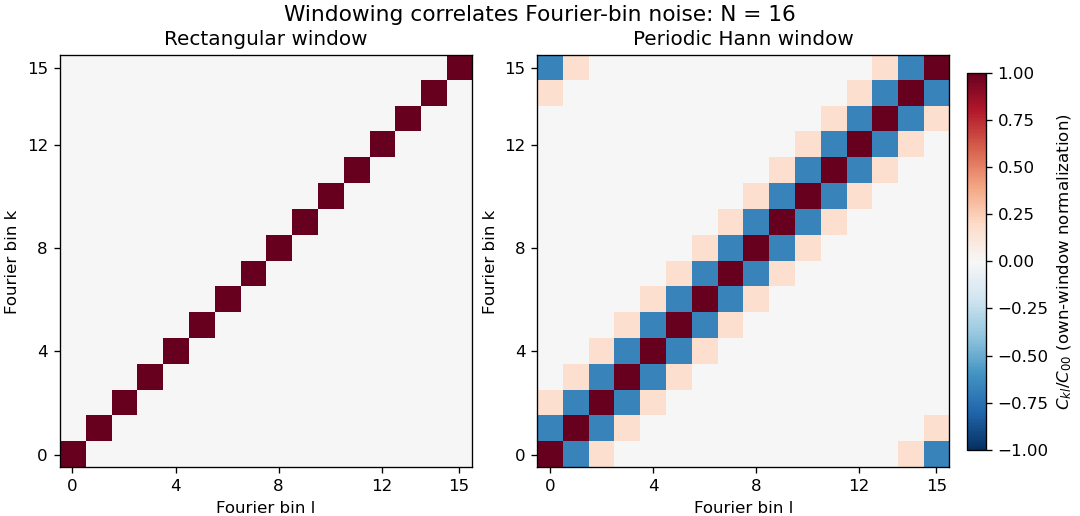
Noise covariance between windowed Fourier bins for rectangular and periodic Hann windows
. Exact original N=16 grid covariance matrices for independent equal-variance sample errors. Each matrix is divided by its own diagonal variance, so the plot compares correlation structure rather than absolute noise level. The corner bands arise from cyclic bin indexing. No sampled experimental data or random simulation is used. Details.Correlation of neighboring periodogram powers is different from the sign of this complex covariance. Suppose each input sample has independent Gaussian real and imaginary parts, each of variance , with all components independent across time. The nonconjugated second moments vanish. Gaussian fourth-moment pairing, as in Isserlis's theorem, then givesConsequently neighboring Hann-bin powers are positively correlated despite the negative covariance of their complex amplitudes. If , their individual power variances are , and the variance of their arithmetic mean isTreating them as independent would incorrectly give . For real Gaussian input, a further term enters the power covariance; the pseudo-covariance of a complex random variable and conjugate-frequency symmetry therefore need attention near paired bins and the real-valued endpoint bins.
Zero padding creates more closely spaced evaluations of the same record, not more independent noise realizations. Even a rectangular record generally has correlated estimates on that denser grid. Detrending, colored input noise and overlapping records change the covariance calculation too. SciPy exposes detrending and FFT-length choices explicitly; its default constant detrending must be disabled when testing the unmodified independent-sample model above.[ref]
A proposed numerical check generates many independent records with the stated noise distribution, computes the estimates with fixed coefficients, and compares empirical complex covariance and power covariance separately with the formulas. A physical noise test additionally needs a characterized acquisition bandwidth and an assessment of time-sample correlation. Averaging several correlated spectral values does not supply the same precision gain as averaging independent records.
The habenula is a small nuclear complex of the epithalamus at the dorsal posterior wall of the third ventricle, adjacent to the dorsal thalamus and pineal gland. In mammals, its medial habenula and lateral habenula are distinct divisions with different circuits. The name denotes neural tissue, rather than a hormone-secreting gland.[ref]
Habenula in NLM MeSH. D019262 scope note: location, habenular nuclei and epithalamic membership.
The distinction between divisions matters when assigning a measured function. In a reward-location reversal task, recordings from the lateral habenula of monkeys showed responses opposing those of dopamine neurons: many lateral habenular cells were more active when an outcome was worse than expected. Weak electrical stimulation of the lateral habenula inhibited recorded dopamine neurons.[ref]
Lateral habenula as a source of negative reward signals in dopamine neurons by Masayuki Matsumoto and Okihide Hikosaka. Nature447,1111–1115(2007), abstract and reward-reversal/stimulation experiments.
For example, if a cue that formerly predicted a reward ceases to do so, the experiment asks whether neural activity follows the new outcome relationship rather than merely the cue's appearance. A change after reversal supports an outcome-related signal. It does not establish that every neuron in the habenula encodes disappointment, nor does electrical stimulation establish a direct single-synapse pathway. Keeping the whole complex, its divisions and the recorded cell populations distinct makes the anatomical term useful when comparing experiments.
The pineal gland is a small neuroendocrine organ of the epithalamus, attached to the roof of the third ventricle. It secretes melatonin, linking a neural timing system to a chemical signal distributed beyond the brain. Its anatomical position is distinct from that of the nearby habenula.[ref]
Pineal Gland in NLM MeSH. D010870 scope note and anatomical hierarchy.
A classic experiment located a strong daily rhythm at an enzymatic step in pineal metabolism. In 1970, D. C. Klein and J. L. Weller reported that rat pineal serotonin N-acetyltransferase activity was more than 15 times higher at night than during the day. The rhythm persisted in complete darkness and in blinded animals, whereas constant illumination suppressed it. Their experiments in isolated tissue also implicated norepinephrine in regulation of the enzyme activity.[ref]
Indole metabolism in the pineal gland: a circadian rhythm in N-acetyltransferase by D. C. Klein and J. L. Weller. Science169,1093–1095(1970), abstract: lighting conditions, enzyme rhythm and in-vitro regulation.
The darkness control is particularly illuminating. A mechanism that merely switched on whenever light was absent would predict a continuously high output in constant darkness. Continued rhythmic variation instead supports an internally generated timing signal. It does not show that the pineal gland alone generates the organism's entire circadian rhythm: the measurement concerns one gland and one metabolic activity in an intact timing system. Likewise, the reported activity ratio is an enzyme-assay result, not a universal ratio of human blood melatonin concentrations.
The temporal energy centroid of an optical pulse is its energy-weighted mean time. For nonnegative radiant power with finite positive energy and finite absolute first moment,The normalization uses radiant energy as integrated radiant flux.[ref]
International Lighting Vocabulary by CIE. entry 17-21-041, note 1
The centroid is a moment of the energy-normalized pulse profile; it need not coincide with the largest power value, a threshold crossing or the middle of the FWHM interval.For an original two-component example, let ninety percent of the energy belong to a symmetric narrow component centred at zero and ten percent to a symmetric component centred at . Linearity of the integral gives . Weak delayed energy can move the centroid even when the dominant peak remains near zero. Multiplying the whole power trace by a positive constant leaves unchanged; translating it by shifts its centroid by .
A detector response can shift the measured centroid too. Suppose a normalized impulse response and normalized optical profile have finite absolute first moments. For their convolution , direct integration with givesThus a causal exponential detector response of time constant shifts the recorded centroid by in this model. NIST's pulsed-radiometer characterization explicitly measures detector impulse responses and uses convolution to assess reproduced waveforms.[ref]
Calibration Service for Low-level Pulsed-Laser Radiometers at 1.06 µm: Pulse Energy and Peak Power by Rodney W. Leonhardt. §§6.1–6.2, printed pp. 13–15
The centroid identity is the independent moment calculation above.Baseline drift can cause a separate shift. Suppose a true pulse has and , but a positive residual baseline of remains across the analysis window from to . Its added energy is , centred at . The resulting centroid isA waveform measurement should therefore record the time window, baseline estimate and detector timing response with its reported centroid. A negative background-subtracted trace also needs care: it is not automatically a nonnegative energy distribution.
Volume normalization of ventricular pressure-volume curves expresses chamber volume relative to a stated reference scale before comparing pressure-volume relations. It can separate the effect of chamber size from differences in the shape of an end-diastolic pressure-volume relationship. It does not automatically remove effects of wall thickness, geometry, external pressure or active state.
Let for fixed positive reference volume , and suppose . The chain rule givesThus equal normalized curves can have different dimensional ventricular compliances. The scaled compliance has units of inverse pressure and compares the same normalized operating point.
For an original example, take mmHg. At , pressure is 1.644 mmHg and mmHg. Chambers with and 200 mL then have volumes 120 and 240 mL and compliances approximately 9.147 and 18.294 mL/mmHg. Their compliances differ by twofold while agrees. These are chosen model chambers, not reference values.
An affine convention must state both its origin and scale . Choosing each curve's reference from the same data can also conceal the very shift being compared. Normalizing every single observation by its own volume makes every normalized volume one and destroys information about curve shape.
An experimental comparison needs independent volume information and a specified pressure reference. The 1994 isolated-heart study used known intraventricular balloon volumes, micromanometer pressure and image-derived ventricular area to compare pressure-volume and pressure-area measurements.[ref]
Estimation of left ventricular compliance using on-line echocardiographic automated border detection and pressure data by John Gorcsan III and others. Abstract, balloon reference, simultaneous imaging/pressure acquisition and validation limitation
That apparatus illustrates why a geometric surrogate must be checked before it becomes the denominator of a normalization.A transparent report identifies the reference volume, whether pressure is intracavity or transmural pressure, the cardiac phase and the operating points compared. A size-normalized chamber curve is still a chamber measurement; it is not by itself a material stress-strain relation for myocardium.
An elliptic fibration is a proper surjective morphism with connected fibres whose generic fibre is a smooth genus one curve. Some conventions additionally require a section of a morphism, which chooses an origin and makes that generic fibre an elliptic curve; the presence of a section should be stated explicitly. Over special points of , fibres may be singular.
For a fixed elliptic curve , projection is an elliptic fibration with constant smooth fibres and a section from the origin of . A nonconstant family can be described on a chart by a Weierstrass equation of an elliptic curve . In characteristic different from two and three, zeros of mark singular cubic fibres, when the displayed family defines the relevant model.
The fibration viewpoint separates the geometry of individual curves from how they vary and degenerate across the base. In dimension two it is the structure underlying an elliptic surface.
The electroretinogram b-wave is a prominent positive-going component of many light-evoked electroretinography traces, associated strongly with the activity of ON retinal bipolar cells. It is an extracellular tissue-level signal, rather than the intracellular membrane potential of one photoreceptor or one bipolar cell. Its appearance and amplitude depend on the stimulus and recording conditions.[ref]
B-wave of the electroretinogram. A reflection of ON bipolar cell activity by Richard A. Stockton and Malcolm M. Slaughter. Abstract: intraretinal fields, pharmacological isolation and ON bipolar contribution.
The assignment was tested by perturbing retinal pathways. In amphibian preparations, APB suppressed ON bipolar responses and removed the b-wave; treatments suppressing OFF-related responses removed the light-offset d-wave while preserving the b-wave. Recording potassium changes along with field responses helped link the electrical component to a specific functional pathway.[ref]
B-wave of the electroretinogram. A reflection of ON bipolar cell activity by Richard A. Stockton and Malcolm M. Slaughter. Selective pharmacological comparisons and extracellular potassium measurements.
A later molecular perturbation supplied independent evidence. Mice lacking TRPM1 retained a normal rod a-wave but lacked the b-wave, while direct bipolar-cell recordings supported disruption of postsynaptic ON signaling. A signal from the early photoreceptor stage can therefore persist when the later response is lost.[ref]
For an illustrative trace, a preceding trough at and a positive peak at are separated by . That trough-to-peak difference differs from the peak's displacement above a zero baseline. Always state the amplitude convention; these invented values are not diagnostic limits or data from either study.
Freeze-fracture electron microscopy reveals structures along a fracture through a frozen specimen, commonly within a biological membrane. The exposed surface is shadowed with a thin platinum-carbon deposit; supporting carbon stabilizes the replica, which is cleaned and examined by transmission electron microscopy. The image is of this replica, not a direct view through the original thick tissue.[ref]
Freeze-fracture electron microscopy by Nicholas J. Severs. Abstract and protocol, fracture, metal-carbon replica and TEM examination
A practical preparation rapidly freezes tissue, fractures it in a cold vacuum apparatus, deposits the replica and transfers the cleaned film to a microscope grid. Membranes often split through their hydrophobic interior, exposing particles and complementary depressions associated with membrane proteins. The fracture plane is not generally the original outer cell surface.
This method is useful because it displays lateral membrane organization that a thin cross-section can hide. However, freezing artifacts, shadowing direction and fracture-path selection affect appearances. Combining replica structure with immunoelectron microscopy can help identify selected proteins, while an unlabeled intramembrane particle should not be assigned a molecular identity from shape alone.
Immunoelectron microscopy uses antibody binding to locate selected molecular targets in an electron microscope image. A common method couples an antibody, directly or through a secondary reagent, to an electron-dense gold particle. The particle supplies visible contrast while the antibody supplies molecular recognition.[ref]
Immunoelectron microscopy by JEOL. Electron-microscopy terminology, antigen-antibody recognition and localization
For example, to ask whether a membrane protein is concentrated in one cellular compartment, label thin sections, count gold markers in that compartment and compare with its area and with background regions. Thirty markers over give a raw density of ten per square micrometre; three over an equal-area negative control give one. That difference is evidence about labeling specificity, not automatically an absolute protein count.
Controls include omitting the primary antibody and testing material lacking the target. Fixation can destroy or hide binding sites, and the antibody-marker complex displaces the visible particle from the target molecule. An unlabeled region may therefore reflect inaccessible antigen rather than absence of the molecule. Molecular specificity and spatial resolution require separate checks.
Immunogold labeling localizes a molecular target using antibody recognition linked to small gold particles, which provide strong contrast in electron microscopy. In an indirect method, a primary antibody recognizes the antigen, and a gold-conjugated secondary antibody recognizes the primary antibody. Recognition supplies specificity; the gold supplies a visible marker.[ref]
Immunoelectron microscopy by JEOL. Technical glossary, indirect primary/secondary antibody method; pre-embedding and post-embedding reactions.
An illuminating application located nephrin near the slit diaphragm between podocyte foot processes. The 1999 study used post-embedding labeling with antibodies against an extracellular nephrin region and a secondary antibody carrying 10-nanometre gold particles. In a tangential section, a row of nine particles lay within a slit approximately 40 nanometres wide. The image supported association with a narrow cellular junction, rather than uniform labeling of every neighboring structure.[ref]
Nephrin is specifically located at the slit diaphragm of glomerular podocytes by V. Ruotsalainen and others. Figure 3A–C and caption: Lowicryl embedding, 10-nm gold and labeled slit; 40 nm describes slit width.
Nine particles do not necessarily mean nine target molecules. Antibody accessibility, labeling efficiency, nonspecific binding and the physical displacement between the recognized site and the particle complicate counting and positioning. A 10-nanometre particle diameter is not automatically a 10-nanometre localization accuracy.
Sampling geometry also matters. An invented comparison of 12 particles along 6 micrometres of membrane and 2 particles along 2 micrometres gives 2 and 1 particles per micrometre, respectively. Raw counts alone would exaggerate the contrast. These are normalized marker densities, not absolute molecular concentrations. The method is most informative when molecular recognition, structural context and appropriate controls agree.
Freeze-fracture microscopy exposes internal structure by breaking a frozen specimen and examining the revealed face with electron microscopy. Freezing makes it possible to prepare a surface through material that would otherwise change substantially during ordinary handling in a vacuum. Physical applications include inspecting internal interfaces in frozen mixtures; the observed face is a fracture-selected surface rather than an arbitrary transparent section.[ref]
Brief Introduction to Freeze Fracture and Etching by Gisela Höflinger. Opening definition and physical preparation discussion, frozen fracture and material interfaces
A preparation workflow freezes the specimen, fractures it while cold, and maintains protected low-temperature transfer. Optional freeze-etching removes surface ice by sublimation under vacuum. A thin oblique metal deposit supplies topographic contrast, with carbon providing support where a replica is required. The prepared block face can be examined with a scanning electron microscope, or a replica can be examined by transmission electron microscopy.[ref]
Brief Introduction to Freeze Fracture and Etching by Gisela Höflinger. Sublimation and condensation discussion; freeze-fracture coating and SEM block-face versus TEM replica routes
A geometrical illustration explains directional shadowing. Model deposition as parallel trajectories making angle above a flat surface. A protrusion of height casts a nominal shadow lengthFor an illustrative , gives , whereas gives about . These are ideal geometric predictions, not measured features or a calibration of a coating instrument. Finite coating thickness, trajectory spread and surface shape affect real contrast.
A useful preparation-control experiment compares otherwise matched frozen samples fractured and coated at different orientations, recording temperature history, etching time and deposition direction. Features that change with coating direction may reflect shadow geometry; features that change with freezing or etching conditions may reflect preparation. The fracture path can favor weak interfaces, and deposited material can obscure small structures, so apparent topography is not automatically an unbiased reconstruction of the original specimen.
The freeze-fracture electron microscopy article describes the replica route in more detail. Here the physical preparation and block-face comparison explain why the microscope image must be interpreted together with the specimen's preparation history.
Serial-section electron microscopy reconstructs a volume from an ordered image stack of thin physical slices. In the transmission electron microscopy implementation, an ultramicrotome cuts successive slices, which are collected on a support and imaged through the specimen. Image registration aligns corresponding features; image segmentation identifies structures to follow between slices. JEOL's glossary describes sections of 40–100 nm and illustrates the separate registration and segmentation stages.[ref]
The motivation is geometrical: one isolated slice cannot show whether a feature continues, divides, or ends outside that slice. An ordered image stack provides observations along the third coordinate, although finite section-thickness anisotropy and missing material limit what can be inferred. A change between neighboring images may come from specimen structure, a slice deformation, or imperfect image registration.
For a chosen numerical example, suppose each of consecutive sections has uniform thickness , with lateral pixel pitch . Ignoring lost material and thickness variation, the sections coverThe voxel sampling is 12.5 times coarser along the cutting direction. These are chosen dimensions, not measurements from either cited experiment. The first and last section centers are only apart: center-to-center extent differs from total represented thickness. Neither spacing is automatically the achieved spatial resolution.
Image resampling onto a cubic grid can make an image stack easier to display, but interpolation supplies no additional independent observations. Likewise, smooth image registration cannot resolve missing-section ambiguity in volume reconstruction: a small connecting feature could lie wholly inside lost material. Checking a reconstructed connection therefore needs evidence in the acquired slices, not just a visually smooth rendered surface.
A historically important automation change illustrates the distinction between section and surface imaging. In 2004, Winfried Denk and Heinz Horstmann placed an ultramicrotome with a diamond knife inside a scanning electron microscope. Their serial block-face scanning electron microscopy imaged the exposed block surface between cuts instead of collecting the removed sections. They reported stacks several hundred layers deep, 50–70 nm sectioning, and typically less than 10 nm lateral position jitter. These observations tested an apparatus for acquiring closely aligned serial images; they did not remove the finite spacing between observations.[ref]
Serial Block-Face Scanning Electron Microscopy to Reconstruct Three-Dimensional Tissue Nanostructure by Winfried Denk and Heinz Horstmann. Abstract; Results, lateral-position stability; Materials and Methods, Microtome
A mechanical detail makes the measurement chain concrete. Their specimen-advance lever reduced the motorized micrometer's motion by 0.11. Thus its stated position measurement uncertainty of 50 nm contributed after that reduction; other sources of section-thickness error still required assessment.[ref]
Serial Block-Face Scanning Electron Microscopy to Reconstruct Three-Dimensional Tissue Nanostructure by Winfried Denk and Heinz Horstmann. Materials and Methods, Microtome, specimen-advance mechanism
An ultramicrotome is a precision cutting instrument for producing very thin sections or successively exposing new specimen faces for electron microscopy. Ultramicrotomy combines a controlled specimen feed with a cutting stroke across a sharp diamond knife or suitable glass knife. A polymer block is one example of a specimen for materials work. JEOL describes preset feeds of tens of nanometres and notes that actual section thickness can differ from the setting.[ref]
Ultramicrotomy by JEOL. Definition, specimen advance and diamond-knife cutting description; thickness dependence on material and temperature
The mechanism must distinguish the feed direction, which sets the intended removed thickness, from the much longer cutting stroke across the block. Section collection supports transmission electron microscopy; an in-chamber version supports serial block-face scanning electron microscopy by imaging the remaining surface.
For an original cutting-budget example, suppose a polymer block is advanced by per cut. After 250 uniform cuts the nominal removed thickness isIf one entire section is lost during collection, its neighbors' centers are apart rather than , assuming all feeds were correct. The total removed thickness remains ; the lost section leaves an observation gap. Recording only the number of surviving images would conceal that gap.
A physical check compares the intended feed with an independent thickness or accumulated-depth measurement, while recording specimen and knife conditions. A fine actuator increment alone does not establish the actual section thickness. Compression, uneven cutting and missing sections affect the geometry subsequently assigned to an image stack.
Serial block-face scanning electron microscopy acquires a three-dimensional dataset by repeatedly imaging an exposed specimen face in a scanning electron microscope and removing a thin layer with an ultramicrotome. The removed layer is not the imaged object: each image records the newly exposed block face. This differs from collecting and imaging thin sections in serial-section electron microscopy.[ref]
Serial Block Face Scanning Electron Microscopy by JEOL. Definition, in-chamber sectioning and imaging of the newly exposed face
In the 2004 apparatus of Winfried Denk and Heinz Horstmann, a diamond knife operated inside the microscope chamber, with controlled specimen advance and retraction. A backscattered electron signal supplied image contrast. Keeping the cutting and imaging operations in the chamber enabled automated image stack acquisition.[ref]
Serial Block-Face Scanning Electron Microscopy to Reconstruct Three-Dimensional Tissue Nanostructure by Winfried Denk and Heinz Horstmann. Results, Block-Face Imaging; Materials and Methods, Microtome
For an original ideal geometry, acquire the first face at , then advance and remove before each subsequent image. An image stack of faces has its last acquired face atThis requires 100 inter-image cuts. If a data format assigns each face a -deep voxel, its nominal represented thickness is instead . State which extent is intended. At lateral pixel pitch , the sampling ratio is 8.
The resulting image stack needs image registration and a calibrated cutting coordinate. Lateral position jitter, cutting artifacts and the depth range contributing to the electron signal limit the useful reconstruction. Finite voxel spacing is not itself a measurement of spatial resolution. Destructive cutting also means that later imaging cannot recover an exposed face that has already been removed.
A difference electron density map is an electron density map calculated to reveal disagreement between measured diffraction amplitudes and those predicted by a crystal structure model. The common map combines observed-minus-calculated amplitude information with phases, usually derived from the model. In practice map coefficients include weighting rather than simply subtracting raw measured intensities.[ref]
Electron Density Maps and Coefficient Files at RCSB PDB. Introduction, difference maps and weighted amplitude/phase coefficient files
For one simplified convention, let . A schematic unweighted difference map isThe crystallographic phases remain necessary even though the coefficients represent differences. Positive features can indicate density missing from the model; negative features can indicate excessive modeled density. Errors in positions, crystallographic site occupancies or atomic displacement parameters can all contribute.
An original one-dimensional idealization takes and , with matching phases. Their difference isIt is positive near0 and negative near , although its integral over one period is zero. Positive and negative residuals therefore need not mean that the total electron count is wrong.
Experimentally the difference electron density map guides corrections to a fitted macromolecular structural model. Finite diffraction data, uncertain phases and model-derived coefficients affect its interpretation; a peak alone does not uniquely identify an atom or chemical species.
The sheet elastocapillary energy ratio compares capillary and bending energy scales for an elastic sheet:Here is a lateral size, is surface tension, is plate bending stiffness and is the elastocapillary length. The ratio is a dimensionless quantity: and both have units of energy.
The estimate assumes bending through an angle of order one over size . Then curvature scales as and integrating the bending energy density over area gives a scale . A comparable change in interfacial area gives a surface energy scale . The same balance underlies the capillary origami study's definition of elastocapillary length.[ref]
For an original calculation, take , and . Then . Doubling alone raises it to 10. Halving thickness at fixed , Young's modulus and Poisson's ratio divides by eight and raises to 20.
Changing all dimensions gives another trend. Write and keep material properties and surface tension fixed. At fixed thickness, ; at fixed aspect ratio , and . Thus halving alone gives one quarter of the initial ratio, while halving both and doubles it.
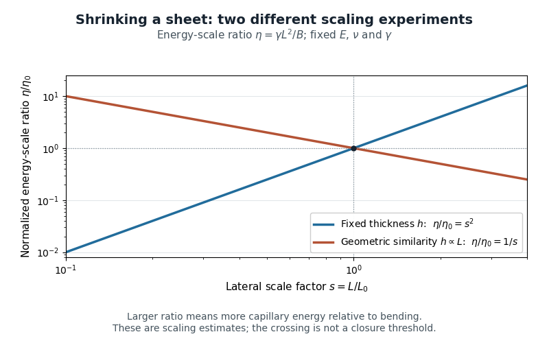
Two size-scaling paths for the sheet elastocapillary energy ratio
. Reuses the original normalized scaling plot: fixed thickness gives , while geometric similarity gives . The curves are dimensional estimates, not measured wrapping thresholds. Details.A larger ratio makes capillary energy more competitive with bending, but does not establish complete closure. Actual wetting, contact angle, droplet volume, contact-line pinning and accessible deformation paths also matter. The ratio compares scales rather than computing the full change in energy along a folding path.
Pinned article: Introduction to the OurBigBook Project
Welcome to the OurBigBook Project! Our goal is to create the perfect publishing platform for STEM subjects, and get university-level students to write the best free STEM tutorials ever.
Everyone is welcome to create an account and play with the site: ourbigbook.com/go/register. We belive that students themselves can write amazing tutorials, but teachers are welcome too. You can write about anything you want, it doesn't have to be STEM or even educational. Silly test content is very welcome and you won't be penalized in any way. Just keep it legal!
Intro to OurBigBook
. Source. We have two killer features:
- topics: topics group articles by different users with the same title, e.g. here is the topic for the "Fundamental Theorem of Calculus" ourbigbook.com/go/topic/fundamental-theorem-of-calculusArticles of different users are sorted by upvote within each article page. This feature is a bit like:
- a Wikipedia where each user can have their own version of each article
- a Q&A website like Stack Overflow, where multiple people can give their views on a given topic, and the best ones are sorted by upvote. Except you don't need to wait for someone to ask first, and any topic goes, no matter how narrow or broad
This feature makes it possible for readers to find better explanations of any topic created by other writers. And it allows writers to create an explanation in a place that readers might actually find it.
Figure 1. Screenshot of the "Derivative" topic page. View it live at: ourbigbook.com/go/topic/derivativeVideo 2. OurBigBook Web topics demo. Source. - local editing: you can store all your personal knowledge base content locally in a plaintext markup format that can be edited locally and published either:This way you can be sure that even if OurBigBook.com were to go down one day (which we have no plans to do as it is quite cheap to host!), your content will still be perfectly readable as a static site.
- to OurBigBook.com to get awesome multi-user features like topics and likes
- as HTML files to a static website, which you can host yourself for free on many external providers like GitHub Pages, and remain in full control

Figure 2. You can publish local OurBigBook lightweight markup files to either OurBigBook.com or as a static website.
Figure 3. Visual Studio Code extension installation.
Figure 5. . You can also edit articles on the Web editor without installing anything locally. Video 3. Edit locally and publish demo. Source. This shows editing OurBigBook Markup and publishing it using the Visual Studio Code extension. 
- Infinitely deep tables of contents:




All our software is open source and hosted at: github.com/ourbigbook/ourbigbook
Further documentation can be found at: docs.ourbigbook.com
Feel free to reach our to us for any help or suggestions: docs.ourbigbook.com/#contact