Laser flash analysis measures thermal diffusivity by heating one face of a specimen briefly and recording the opposite face's temperature rise. The original 1961 experiment used a flash tube rather than a laser: a blackened thin metal specimen sat in an opaque ceramic holder, with thermocouple wires pressed against its rear face. An amplifier, oscilloscope and camera recorded the signal. Uniform front illumination and the black coating promoted uniform absorption; the opaque low-thermal conductivity holder blocked direct rear illumination and reduced edge losses. The delayed rear response reveals internal thermal conduction rather than direct heating of the sensor. ^[ref]

A modern version uses a laser or flash lamp, a specimen of measured thickness $L$, controlled initial temperature, and a rear-facing infrared detector with a synchronized recorder. The readout is a temperature rise versus time, starting from a pre-pulse baseline. Thermal conductivity additionally requires mass density and specific heat capacity; it is not obtained from timing alone. ^[ref]

Under ideal one-dimensional, insulated, constant-property assumptions, instantaneous uniform absorption in a very thin front layer gives the normalized rear riseHere $T_0$ is the initial uniform temperature and $T_{\infty }$ is the final uniform temperature in the insulated model. Fitting this curve estimates thermal diffusivity; each term has the same $\alpha K_n^2$ decay as the insulated-bar Fourier modes. Equivalently, the half-rise time $t_{1/2}$ solves $R(t_{1/2})=1/2$. Writing $s=\alpha t/L^2$, the series gives $s_{1/2}\approx 0.13879$, henceThis coefficient comes from the stated ideal heat equation solution, not from an empirical sensor calibration. It has been independently checked by solving the series equation. Absolute absorbed pulse energy cancels from the normalized curve; determining heat capacity from its absolute height needs additional information. ^[ref]

Parker and colleagues identify finite flash duration, heat loss, nonuniform illumination, recording bandwidth and electrical interference as practical limits. A specimen too thin responds during the pulse; one too thick allows losses before the rear rise finishes. They shielded the electrical chain and recorded a baseline; their reported tests were preliminary metal measurements near ambient and moderately elevated temperatures. ^[ref]

Useful additional controls are to measure thickness at several points, verify the recorder's time scale and detector response independently, record a no-pulse baseline, and repeat at different pulse energies while avoiding phase transitions. Compare different thicknesses of the same homogeneous material: ideal half-rise times scale as $L^2$. Failure of these checks can expose finite-pulse effects, sensor delay, optical transmission, coating storage or edge losses; a thickness error is especially consequential because the inferred thermal diffusivity depends on $L^2$. These are proposed diagnostic controls, not invented measurements. When the pulse is not short or the sample exchanges appreciable heat with its surroundings, fit a model that includes those effects instead of applying the ideal half-rise coefficient unchanged.

An adiabatic wall prevents heat transfer. Two bodies at $300\mathrm{K}$ and $350\mathrm{K}$ can remain separated by a rigid adiabatic wall with no heat transfer, although they are not in thermal equilibrium with each other. An adiabatic boundary alone need not make a system an isolated system: a moving insulated piston can still transmit work. Isolation additionally excludes matter transfer and every energy exchange.

A diathermal wall permits heat transfer. For a clean zeroth law of thermodynamics comparison, idealize it as rigid and impermeable, excluding boundary work and matter transfer. A thin metal partition approximates this arrangement.^[ref]

Set $n=(3^s-1)/2$ and let $\beta$ be a primitive element of a finite field ${\mathbb{F}}_{3^s}$. The powers $1,\beta ,\dots ,{\beta }^{n-1}$ represent every projective point once. Their kernel code is a ternary Hamming code. Since ${\beta }^n=-1$, its polynomial description is a negacyclic code, generated by the minimal polynomial of an algebraic element $\beta$ over ${\mathbb{F}}_3$.

For odd $s\ge 3$, put $n=(3^s-1)/2$ and choose $\alpha$ of order $n$ in ${\mathbb{F}}_{3^s}$. Because $n$ is odd, the powers ${\alpha }^i$, $0\le i<n$, represent every projective point once. The cyclic code defined by $c(\alpha )=0$ is therefore monomially equivalent to a ternary Hamming code, with the displayed generator polynomial of a cyclic code. This statement requires a qualification: at $s=2$, every ternary cyclic length-four, dimension-two code has a weight-two generator, so none has Hamming distance three.

For an external loop flux $Kz$, positive current orientation and upward Lorentz force $KI$, including self-inductance gives $\mathcal{L}\dot{I}+RI=-K\dot{z}$ and $m\ddot{z}=-mg+KI$. At zero resistance total linked flux is conserved. If initially $I=0$ at $z=z_0$, then $I=-K(z-z_0)/\mathcal{L}$ and the mechanical motion is an undamped oscillator about $z_0-mg\mathcal{L}/K^2$. The finite-resistance terminal speed tends to zero as $R\to 0$, but neglecting self-inductance is a singular approximation in that limit. A lossless loop does not dispose of energy through Joule heating.

Nonnegative tensor-product surface basis factors yield nonnegative product weights. Their two partition of unity sums multiply to one. If the factors are $C^r$ and $C^s$, mixed derivatives through separate orders $r,s$ are continuous, so the resulting finite or locally finite surface representation is jointly $C^{\min (r,s)}$. Control coefficients can cancel derivative jumps and yield more smoothness; inherited continuity is a guaranteed lower bound, not a claim that every surface has exactly the basis's worst regularity.

The splitting principle for complex vector bundles makes pullback injective in integral cohomology and splits both bundles into lines with Chern roots $x_1,x_2$ and $y_1,y_2$. The tensor product has roots $x_i+y_j$. Expanding their six pairwise products gives the displayed formula. This integral computation does not divide by two, so it remains valid when the cohomology has two-torsion. In particular, taking $F$ trivial gives $c_2(E\oplus E)=c_1(E{)}^2+2c_2(E)$.

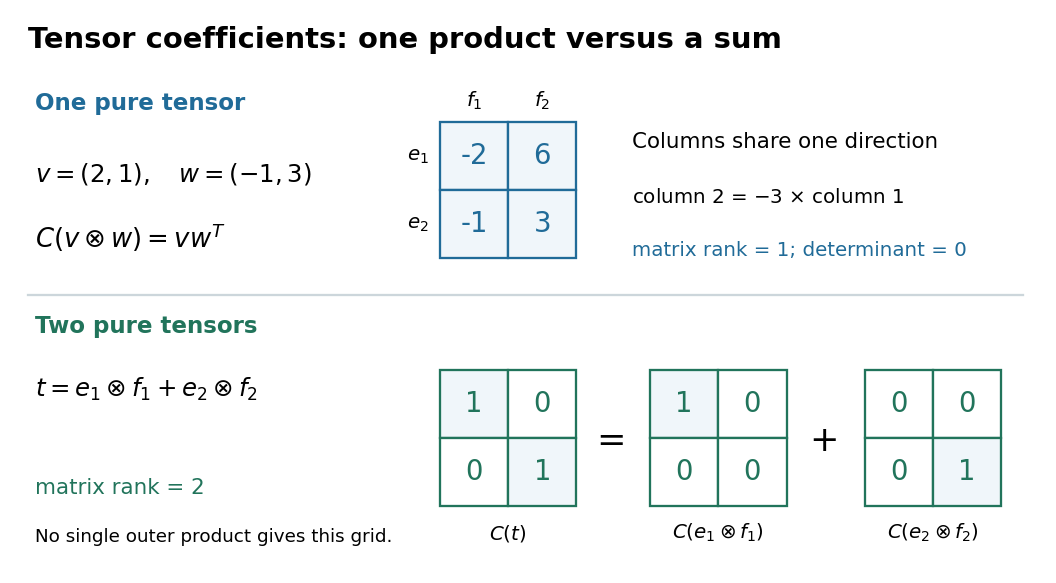
After choosing ordered bases, identify a tensor $t={\sum }_{i,j}{c}_{ij}{e}_i\otimes f_j$ with its matrix $C(t)=(c_{ij})$. This is a linear isomorphism between $V{\otimes }_{F}W$ and the vector space of $m$-by-$n$ matrices: each tensor-product basis element becomes the matrix with one entry equal to one and all others zero. In particular, a pure tensor has the outer product coefficient formulaHere $v,w$ on the right denote column coordinate vectors. The identification depends on the chosen bases, while the tensor itself does not. Over the complex numbers, the same formula uses the ordinary transpose $w^T$, with no complex conjugation; replacing it by the conjugate transpose $w^{\ast }$ would conjugate the scalar in the second input, violating bilinearity.

The truncated tensor algebra discards products of degree greater than $N$. Its multiplication is $(a\otimes b{)}^{(k)}={\sum }_{j=0}^k{a}^{(j)}\otimes b^{(k-j)}$. Every element with scalar part $1$ is invertible by a finite geometric series in its positive-degree part. Over a field of characteristic zero, truncated exponential and logarithm are finite polynomials. More generally, their coefficient formulas require the relevant denominators through degree $N$ to be invertible in the coefficient ring.

A Michelson interferometer divides light at a beam splitter, reflects the two arms at mirrors and recombines the returning fields. For vacuum arm lengths ${\ell }_1,{\ell }_2$, the delay magnitude is $|\tau |=2|{\ell }_2-{\ell }_1|/c$. At each coarse delay, a small mirror scan produces maxima and minima of the detected light intensity. A photodiode and its electrical readout resolve these changes; the scan should cover several carrier cycles while changing $|g^{(1)}|$ negligibly. MIT's laboratory guide uses a mirror actuator, photodiode and electrical drive to scan interference fringes and extract interferometric visibility.^[ref]

A verified motivating experiment is Shaoul Ezekiel's MIT demonstration of source-spectrum control. A polarizer selects one or several lines from a laser whose adjacent lines have orthogonal linear polarizations. A sampled beam goes to a scanning Fabry–Pérot interferometer to check the optical spectrum; the main beam enters a Michelson interferometer, and a lens projects its interference fringes onto a screen. With one selected line the fringes retain good contrast through the demonstrated delay range. With several lines their contrast falls and returns as the arm length changes. At a fixed delay with poor contrast, selecting one line restores it; at matched arms both selections give good contrast. This control isolates the role of spectral composition rather than simply the arm position. The presentation is a qualitative demonstration, not a calibrated linewidth measurement. ^[ref].

A deliberately simpler two-line model explains the return of contrast. Take two stationary, mutually uncorrelated monochromatic contributions of equal power at ${\nu }_0\pm \delta \nu /2$. Their normalized wave-field correlation isfor equal detected single-arm light intensities. At $\tau =1/(2\delta \nu )$ the two contributions' interference fringes cancel on averaging; at $\tau =1/\delta \nu$ they agree again. This is a deduction from the stipulated spectrum, not a fit to Ezekiel's two- or three-line source. Finite individual linewidths eventually damp these revivals.

For a quantitative version of the experiment, the visibility law suggests explicit controls. Measure each arm separately at every coarse delay, subtract the detector's dark signal and any measured background, then normalize by $2\sqrt{I_1{I}_2}/(I_1+I_2)$. Keep the returning beams aligned on the same detector region with parallel linear polarizations; keep detector gain fixed and avoid saturation. Resolve the small mirror scan electrically, rather than averaging over its moving interference fringes. Repeat scans to identify vibration or drift. These controls follow from the averaging and mode-matching assumptions in first-order optical coherence; loss of contrast alone cannot distinguish source decorrelation from apparatus motion, misalignment or insufficient spatial resolution. The finite travel range gives access only to a finite range of delays.

The practical gain is that wave interference measures field correlations even when the detector cannot follow the optical oscillation itself. A long optical coherence length allows unequal-arm measurements; a short one localizes high contrast near matched delays. The beautiful feature is that both fading and reappearance of interference fringes are sums of the same rotating complex amplitudes.

An optical coherence time summarizes the delay scale of temporal optical coherence, but requires a convention. Two useful choices are the first positive delay ${\tau }_{1/e}$ where $|g^{(1)}|=e^{-1}$, for a monotonically decaying envelope, and the integral definitionThe latter counts correlation over both signs of delay and may diverge for ideal discrete lines. ^[ref].

For the stipulated Lorentzian and Gaussian profiles in temporal optical coherence, direct substitution and a Gaussian integral giveThe respective dimensionless coefficients are $0.318310$ for both Lorentzian conventions, and $0.530021$ and $0.664282$ for the Gaussian conventions. The familiar scale $1/\Delta \nu$ is consequently an estimate, not a convention-independent equality. A source with narrow discrete lines can have repeated revivals instead of one monotonically decaying envelope, so recording the full $|g^{(1)}(\tau )|$ can be more informative than one optical coherence time.

For the telescoping series ${\sum }_{n=1}^{\infty }1/[n(n+1)]=1$, the remainder after the first $N$ terms is exactlyThus $S_9=0.9$, $S_{99}=0.99$, and $S_{999}=0.999$. This supplies an exact stopping rule: to make the absolute error at most $10^{-3}$, 999 terms suffice. Requiring strictly less than $10^{-3}$ instead needs at least 1000 terms.

The next term, $a_{N+1}=1/[(N+1)(N+2)]$, is smaller than the full remaining sum by a factor of $N+2$. For example, after 99 terms the next term is $1/10100$, while the remainder is $1/100$. The term test for divergence concerns individual terms; a reliable numerical approximation needs a bound on the whole remaining sum.

A Taylor series centred at zero. Its coefficients are the derivatives there divided by the corresponding factorials.

For a regular real mode between rigid boundaries, multiply the Taylor–Goldstein equation by its vertical structure and integrate to get the stationary quotient $k^2=\int ({\ell }^2{\varphi }^2-{\varphi }_z^2)dz/\int {\varphi }^{2}dz$. Along a differentiable dispersion branch, stationarity removes the variation of the eigenfunction, giving $2k=(\partial I/\partial c)dc/dk$. Since ${\partial }_c{\ell }^2=N^2/(U-c{)}^3+{\ell }^2/(U-c)$, the displayed group velocity follows from $d(kc)/dk$. Critical levels and vanishing branch derivatives require a separate limiting analysis.

For two-dimensional flow under the Boussinesq approximation with $u={\psi }_z$, $w=-{\psi }_x$, a linear mode whose Laplacian is proportional to its streamfunction has zero self-advection of vorticity. Its buoyancy anomaly is $\sigma =a(z)\varphi$, with $a=N^2/(U-c)$. Self-advection of buoyancy vanishes only when the displayed Jacobian is zero. Constant stratification and constant flow make $a$ constant and yield finite-amplitude exact wave solutions. A varying polarization coefficient generally creates a second harmonic, even when the vorticity self-interaction vanishes.

For positive background velocity $U=U_0{e}^{Mz}$ and buoyancy frequency $N=N_0{e}^{Mz}$, a stationary nonzero-horizontal-wavenumber Taylor–Goldstein equation reduces to the displayed constant-coefficient equation. Its structures are oscillatory, affine or exponential according to the sign of $N_0^2/U_0^2-M^2-k^2$. The disturbance Laplacian is a constant times its streamfunction, but its buoyancy anomaly is $N_0^2{e}^{Mz}\varphi /U_0$. Therefore vorticity self-advection vanishes while buoyancy self-advection produces a nonzero second harmonic for $M\ne 0$. These nontrivial real linear modes are not exact finite-amplitude solutions without additional fields. For $M=0$, both polarizations are constant and these nonlinear self-interactions vanish.

A divergence-free magnetic field satisfying the Taylor constraint on all geostrophic cylinders. It is a compatibility condition for slow rotating-fluid balance, not a local force-free condition. To retain such a state as magnetic induction proceeds, the velocity must also preserve the time derivative of the cylindrical torque constraint.

For an instantaneous magnetostrophic Taylor state, the momentum equation leaves a geostrophic null component $u_g=s\omega (s)\hat{\varphi }$. Decompose the velocity into this component and a particular ageostrophic flow, substitute the induction equation into the displayed derivative constraint, and solve the resulting linear equation for $\omega$ with magnetic boundary conditions imposed. When magnetic surface torque vanishes, the geostrophic part is ${\mu }_0^{-1}{\partial }_s[s^3{\int }_{C_s}{B}_s^{2}d\varphi dz{\omega }^{\prime }]$. Boundary terms generally cannot be discarded for an insulating exterior; the primary analysis is Hardy and collaborators' boundary-compatible geostrophic-flow construction. Regularity and an angular-momentum normalization fix remaining homogeneous freedoms when the magnetic coupling is nondegenerate.

With small viscosity, the azimuthal cylindrical balance permits Lorentz force torque to be cancelled by viscous stress. For ordinary no-slip rotating boundaries an Ekman layer gives stress of order $\rho \Omega LU\sqrt{E}$, larger than the order-$E$ bulk viscous correction at fixed velocity. Thus bounded small-$E$ flows approach a magnetostrophic Taylor state but need not satisfy its constraint exactly at finite viscosity. An order-one uncompensated magnetic torque would require a divergent flow as $E\to 0$, invalidating the assumed small-inertia balance. Stress-free boundaries remove the leading no-slip friction and require their own torque/regularity conditions.