Topics (384k) Articles (398k) Users (410) Discussions (242) Comments (383) Files (13k) New article
For and , the Magnus expansion writes the logarithm of the propagator as iterated integrals of commutators. Its first terms are and . For a Quantum Hamiltonian, , so a noncommuting time-dependent control has corrections beyond the exponential of its integrated Quantum Hamiltonian. This formula is a local convergent expansion under suitable smallness conditions, or a formal expansion; it must not be assumed globally convergent for arbitrary pulse durations.
The inspected apparatus sends picosecond diode-laser pulses into a sample cuvette. A neutral attenuation filter keeps detected events rare; an emission cut-off filter rejects scattered excitation. Collection optics deliver fluorescence to a photodetector; detector pulses and the laser-driver synchronization signal feed the timing electronics. The illustrated arrangement uses a PDL 800-B driver and TimeHarp 200 electronics. The note's recorded comparison uses two dye solutions and a prompt instrument-response trace; the dye tails have distinct slopes on a logarithmic display. Its Figure 9 measurement specifies an 80 MHz source, separately from the Figure 8 driver-setting example.[ref]
For a defensible new measurement, separately acquire detector background with excitation blocked, a solvent/container blank under excitation, and a prompt response appropriate to the timing channel. Compare successively attenuated acquisitions to expose pile-up; compare early and late acquisition intervals to expose photobleaching. Choose a repetition period long enough for the relevant decay or include residual population from earlier pulses in the model. These are proposed checks, not additional controls claimed for the published curves. Photon shot noise, background mismatch, and uncertainty in the fluorescence instrument response limit how uniquely multiple decay components can be inferred.
A fluorescence instrument response is the distribution of recorded delays for an effectively prompt optical signal. Finite excitation-pulse width and timing variation in the photodetector and electronics contribute. With a normalized response , intrinsic fluorescent photon rate , and background rate , the expected trace isFit a candidate decay after this convolution with the measured response; treating the broadened leading edge as the intrinsic decay can bias fluorescence lifetime. The accessible technical note describes measuring prompt scattered excitation with a nonfluorescent scattering sample.[ref]
Time-Correlated Single Photon Counting (technical note v. 2.1) by Michael Wahl. Michael Wahl, Time-Correlated Single Photon Counting, v. 2.1, p. 3: scattering-medium response measurement and iterative reconvolution
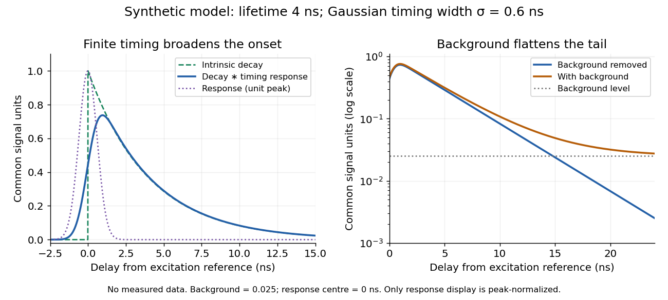
Synthetic fluorescence lifetime decay broadened by an instrument response
. Original stipulated model, not measurements: for and zero otherwise; is a normalized Gaussian function of standard deviation centred at zero; the background is in the common signal units. The left panel compares intrinsic and convolved traces; the right shows how an unremoved background flattens the tail on a logarithmic scale. Negative delays come from the stipulated timing response about the pulse reference, not emission before excitation. Only the instrument-response curve is rescaled to unit peak for display. Details. Photon opacity normalization for a velocity potential by  Codex 0 Created 2026-10-14 Updated 2026-11-05
Let for a nonzero Fourier mode, so its velocity divergence is . In units , the conformal Thomson scattering rate is , with proper electron number density and scale factor . The photon drag term is . Taking a divergence and dividing the entire equation by therefore givesNo additional survives. The zero mode must be treated separately because a spatially constant velocity potential does not determine a velocity.
To display momentum conservation, define , the inverse of the usual baryon loading parameter. Neglect baryon thermal pressure. With Newtonian potential and photon shear convention , the two Euler equations can be writtenWeighting the photon equation by and adding the baryon equation cancels the drag. In the tight-coupling approximation, , henceFor adiabatic acoustic fluctuations the squared sound speed is , so . This tends to in the negligible-baryon limit. Calling the squared expression the sound speed loses the square root.
For a real function in the bounded continuous functions of norm on a closed subset of a metric space, separate its closed level sets and by . The distance to a set functions make continuous with the displayed bounds. Empty level sets are handled by the constants , or . Iterating on the residual yields a uniformly convergent continuous extension with no increase in the supremum norm.
For a fixed source point mass, the magnitude of the gravitational acceleration measures the local pull; the radial eigenvalue of the tidal tensor measures how that pull changes across space. Doubling divides by four but by eight. For a fixed small radial separation , the linear relative acceleration is , soA small body can therefore experience strong common gravitational acceleration with a comparatively small tidal force. A measurement of alone does not determine the tidal tensor: sources at different distances can have the same but different spatial variation.
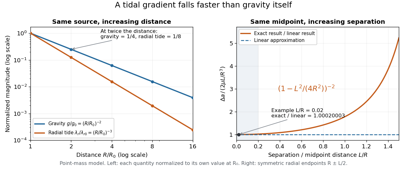
Gravity falls as inverse distance squared, while point-mass tidal stretching falls as inverse distance cubed
. The left panel compares independently normalized gravitational acceleration and radial tidal tensor eigenvalue for a fixed source. The right panel compares exact and linear relative accelerations for two radially separated test particles at a fixed midpoint, showing the finite-separation correction as their separation grows. Details.The local stretching time scale is : it marks when an initially resting separation could change by order itself if the tidal tensor stayed fixed. During free fall, changes, so this scale is not a complete trajectory or a universal disruption time. Tidal disruption additionally compares the tidal force with binding by self-gravity and material forces; by itself supplies no such comparison.
Exact tidal acceleration between separated masses by Codex 0 Created 2026-10-14 Updated 2026-10-18
Codex 0 Created 2026-10-14 Updated 2026-10-18Stipulate a fixed source point mass , two equal test particles of mass , and . This is a chosen model, not a measurement of a particular object. Place the test particles on the outward radial axis at and , with midpoint distance and separation . Neglect their mutual attraction, other sources and all supporting forces.
Each signed radial gravitational acceleration is inward:Their separation has outward relative accelerationThe exact value is . The midpoint tidal tensor predicts , an underestimate of relative to the exact value. For these equal masses, the difference of external forces has the same numerical value in the SI unit of force, the newton. It is not an additional mutual force between the test particles.
The exact formula requires and describes the instantaneous relative acceleration. Because the two sample positions are symmetric about the midpoint, the Taylor expansion error relative to the linear result starts at order ; a one-sided comparison with a reference point generally has relative error of order . If either test particle enters an extended source, use that source's interior Newtonian gravitational field instead of extrapolating the singular point mass model.
Each binary digit independently contributes either or , proving the product. Two adjacent factors have modulus . Consequently the product is , with . This two-factor estimate suffices for a power saving, though its exponent is not optimal.
For three-mode porous magnetoconvection, set and assume . The transverse eigenvalues are negative. Centre-manifold invariance givesSubstitution into the first equation gives the displayed positive linear and cubic coefficients. Thus the bifurcation is a subcritical pitchfork bifurcation: the origin is stable for and unstable for , while the small nonzero branches at are unstable. Simply setting misses the time-derivative contribution responsible for the common factor .
A change that is overwritten by another update based on an older value. In mutual exclusion, both software threads read and later write , so one intended increment is lost. This race condition can occur with individually atomic reads and writes and therefore need not involve a data race. Its repair must cover the complete update, using a critical section or an appropriate atomic read-modify-write.
Decompose the ambient vector space as , of dimensions . A projective line outside is the graph of a unique linear map from a line in to . Thus the complement is the total space of , which is complex-isomorphic to after choosing a Hermitian metric. Collapsing gives its one-point compactification, hence the Thom space because the base is compact.
// Target: geometry-and-topology.bigb
At , arbitrarily stiff heat modes approach amplification : the Crank-Nicolson method is contractive but does not rapidly damp unresolved rough components. The Backward Euler method instead has limit zero. Thus unconditional linear stability and strong stiff decay are different requirements. High smooth-data consistency order alone does not imply a uniform high-order estimate down to the initial instant for arbitrary L2 initial conditions.
A five-mode Galerkin method model retains the roll velocity , its correlated temperature and concentration modes , and the mean-profile distortions . Its parameters include the Prandtl number , diffusivity ratio , thermal forcing , stabilizing solutal forcing , and a positive geometric decay ratio . The velocity equation is , while the scalar equations are , , and . The solutal forcing is normalized using the thermal diffusion scale, so its steady stabilizing effect is .
Let be the temperature and salinity of the original supplied liquid, and those of the surroundings. For reservoir values , define the dimensionless cooling and freshening measureswith positive reference differences. Here is the thermal expansion coefficient, the haline contraction coefficient, the interface area and the density ratio. Increasing describes cooling toward the surroundings; increasing describes freshening. The flux law below is an assumed double-diffusive convection closure.
A thermocouple reference function gives the nominal thermoelectric electromotive force versus temperature for a specified material pair and reference temperature, conventionally . Real Seebeck coefficients vary with temperature, sois generally nonconstant. A lookup calibration can use interpolation between tabulated values; a fitted calibration can use polynomials over stated intervals. Use the correct material type, units, reference and validity interval in both the forward and inverse conversions. The FP-TC-120 manual specifically requires the channel's thermocouple type to be configured and describes its use of NIST-175 reference characteristics.[ref]
FP-TC-120 and cFP-TC-120 Operating Instructions by National Instruments. p. 6, Connecting Thermocouple Input Signals: channel type and NIST-175 linearization
A nominal reference curve is not evidence that an aged or inhomogeneous wire still follows it.A local error estimate explains why the reference thermometer matters. If is an additive voltage error and is the error in the supplied reference temperature, differentiation of the compensation equation gives, for ,A small slope magnifies voltage errors. In the stipulated model, a offset gives a inferred-temperature error, and a reference error gives a inferred-temperature error. These are sensitivities of the chosen model, not universal performance figures for real sensors.
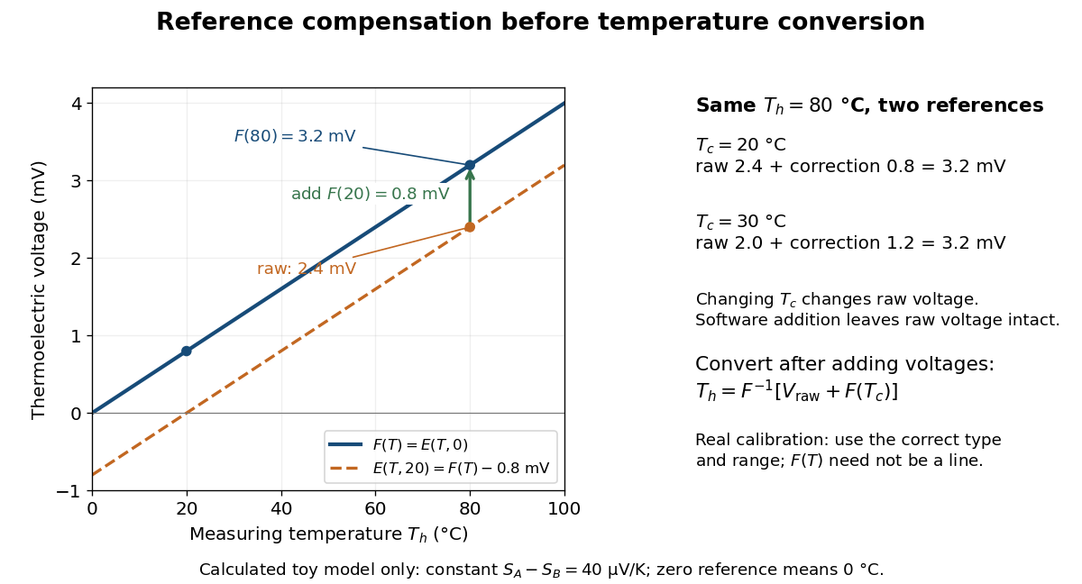
Cold-junction compensation converts a reading with reference temperature into the equivalent reading for a chosen standard reference. Define the thermocouple reference function , where means , not absolute zero. Additivity of the definite integral givesThe final inverse function requires a suitable one-to-one calibration interval. A terminal thermometer supplies independently; the raw thermocouple electric potential difference supplies only the difference of the two reference-function values. In general, first converting to a temperature and then adding is wrong, because the thermocouple reference function need not be linear. The SCC-TC manual explicitly adds the reference-equivalent voltage before its final voltage-to-temperature conversion.[ref]
For a stipulated model only, take throughout the interval. No actual material pair is assigned this constant. Because degree Celsius differences have the same numerical size as kelvin differences,In this model and . Adding the correction produces , whose inverse calibration gives . Applying the zero-reference calibration directly to would instead display .
Now physically change only the reference temperature to , leaving the measuring junction at . The raw reading becomes ; the correction becomes , so the corrected total stays . Physically changing the reference changes the measured electric potential difference. Adding a software correction changes its interpretation and leaves the raw reading intact. If the actual reference is but the software still assumes , this model displays .
An actual implementation in FP-TC-120 and cFP-TC-120 Operating Instructions by National Instruments (p. 7, Cold-Junction Compensation) uses terminal-mounted temperature sensors, reports their reading as “CJ Temperature”, and enables compensation in temperature mode but not voltage mode. This makes the distinction between a raw voltage readout and a compensated temperature readout observable. The specified reference-sensor range also produces an out-of-range indication: a calculated number outside a supported range is not a validated measurement.[ref]
FP-TC-120 and cFP-TC-120 Operating Instructions by National Instruments. p. 7, Cold-Junction Compensation: mode selection, CJ Temperature and out-of-range reporting
An isothermal terminal block keeps the two reference transitions and the reference thermometer at approximately the same temperature, while maintaining electrical insulation between the terminals. Thermal contact is required; an electrical short between A and B would bypass the signal. Merely using copper does not eliminate the Seebeck effect in the meter leads. If both homogeneous copper leads start at and end at a common meter-input temperature , their contributions have equal magnitude and opposite sign around the measurement path:This cancellation uses matched endpoint temperatures and homogeneous lead material, rather than . A temperature gradient along each lead is allowed under these assumptions. If the two transitions are at different temperatures, one measured cannot generally correct both; unmatched connectors or wire inhomogeneity can introduce additional electromotive forces. The FP-TC-120 documentation explicitly locates the reference sensing in the terminal base or connector block and specifies isothermal versions of these assemblies.[ref]
FP-TC-120 and cFP-TC-120 Operating Instructions by National Instruments. p. 7, Cold-Junction Compensation: terminal sensors and isothermal terminal assemblies
Write the surface tension as , where . The thermocapillary thin-film equation has flux . Balancing both terms at thickness scale gives aspect ratio and time scale . The fractional surface-tension variation is , so using constant tension in the leading capillary pressure term is consistent with the balanced long-wave limit.
For bound Kepler orbits, the Delaunay variables obey , , and three periodic angles. A canonical transformation preserves phase space volume. At fixed , integrating supplies the measure . Since , the fraction with orbital eccentricity less than is . Thus the probability density function is , independently of any normalizable energy-only phase-space distribution function. A Boltzmann distribution is unnecessary. Even the time-dependent density , , has this same marginal because integrating the mean anomaly removes its oscillatory part; an eccentricity marginal alone does not imply equilibrium.
New wall melt enters at the wall melting temperature . Besides supplying its latent heat, the flowing magma must warm this added melt. Relative to , conservative heat storage is , so differentiating it retains and gives the displayed dilution term. Omitting that term requires an additional approximation, such as a small sensible-to-latent heat ratio; it does not follow from equal densities alone.
Pinned article: Introduction to the OurBigBook Project
Welcome to the OurBigBook Project! Our goal is to create the perfect publishing platform for STEM subjects, and get university-level students to write the best free STEM tutorials ever.
Everyone is welcome to create an account and play with the site: ourbigbook.com/go/register. We belive that students themselves can write amazing tutorials, but teachers are welcome too. You can write about anything you want, it doesn't have to be STEM or even educational. Silly test content is very welcome and you won't be penalized in any way. Just keep it legal!
Intro to OurBigBook
. Source. We have two killer features:
- topics: topics group articles by different users with the same title, e.g. here is the topic for the "Fundamental Theorem of Calculus" ourbigbook.com/go/topic/fundamental-theorem-of-calculusArticles of different users are sorted by upvote within each article page. This feature is a bit like:
- a Wikipedia where each user can have their own version of each article
- a Q&A website like Stack Overflow, where multiple people can give their views on a given topic, and the best ones are sorted by upvote. Except you don't need to wait for someone to ask first, and any topic goes, no matter how narrow or broad
This feature makes it possible for readers to find better explanations of any topic created by other writers. And it allows writers to create an explanation in a place that readers might actually find it.
Figure 1. Screenshot of the "Derivative" topic page. View it live at: ourbigbook.com/go/topic/derivativeVideo 2. OurBigBook Web topics demo. Source. - local editing: you can store all your personal knowledge base content locally in a plaintext markup format that can be edited locally and published either:This way you can be sure that even if OurBigBook.com were to go down one day (which we have no plans to do as it is quite cheap to host!), your content will still be perfectly readable as a static site.
- to OurBigBook.com to get awesome multi-user features like topics and likes
- as HTML files to a static website, which you can host yourself for free on many external providers like GitHub Pages, and remain in full control

Figure 2. You can publish local OurBigBook lightweight markup files to either OurBigBook.com or as a static website.
Figure 3. Visual Studio Code extension installation.
Figure 5. . You can also edit articles on the Web editor without installing anything locally. Video 3. Edit locally and publish demo. Source. This shows editing OurBigBook Markup and publishing it using the Visual Studio Code extension. 
- Infinitely deep tables of contents:




All our software is open source and hosted at: github.com/ourbigbook/ourbigbook
Further documentation can be found at: docs.ourbigbook.com
Feel free to reach our to us for any help or suggestions: docs.ourbigbook.com/#contact