Topics (384k) Articles (398k) Users (410) Discussions (242) Comments (383) Files (13k) New article

Pedigree peeling eliminates latent genotypes by moving sums inside products whenever the other factors do not depend on the eliminated genotype. For one parent genotype and one child genotype , the likelihood becomesThe inner bracket is the child's message to its parent. With two states each, it needs four multiplications and two additions; multiplying the two parent weights and messages needs four more multiplications and the final sum one addition. The unrearranged four terms instead use twelve multiplications. Larger pedigrees use the same variable-elimination identity, with additional handling of pedigree loops.
Assign one genotype random variable to each person in a pedigree. Independent founders in a pedigree carry population genotype laws, and each other genotype has its conditional distribution given its two parents from Mendelian segregation. The ancestry directed acyclic graph is a Bayesian network for the joint genotype law. Its moral graph contains each parent-child edge and each coparent edge. Each founder factor and each child-with-parents factor belongs to a clique, giving an undirected graphical representation. The graph is an independence representation; equality with the minimal conditional independence graph needs additional faithfulness assumptions, particularly because inheritance can produce zero probabilities.
An unphased multilocus genotype can have several pairs of haplotypes. Its pedigree likelihood must average over these possible phases with prior weights , rather than maximize over phases after observing the offspring. Under linkage disequilibrium, the weights need not be equal. They can be obtained by conditioning biological population haplotype frequencies on the observed parental genotype; different choices of what is conditioned on change only parameter-independent factors when those frequencies are held fixed.
A Pauling bond-energy excess subtracts a chosen like-atom baseline from the unlike-atom bond-dissociation energy. For an unequal-input arithmetic example, stipulate , and , all with one dissociation convention. The arithmetic mean baseline and excess areThe arithmetic-baseline Pauling scale model therefore gives . The bond-dissociation energy is not itself the excess: subtracting the baseline is essential. All three numbers are stipulated, not experimental values for named chemical elements.
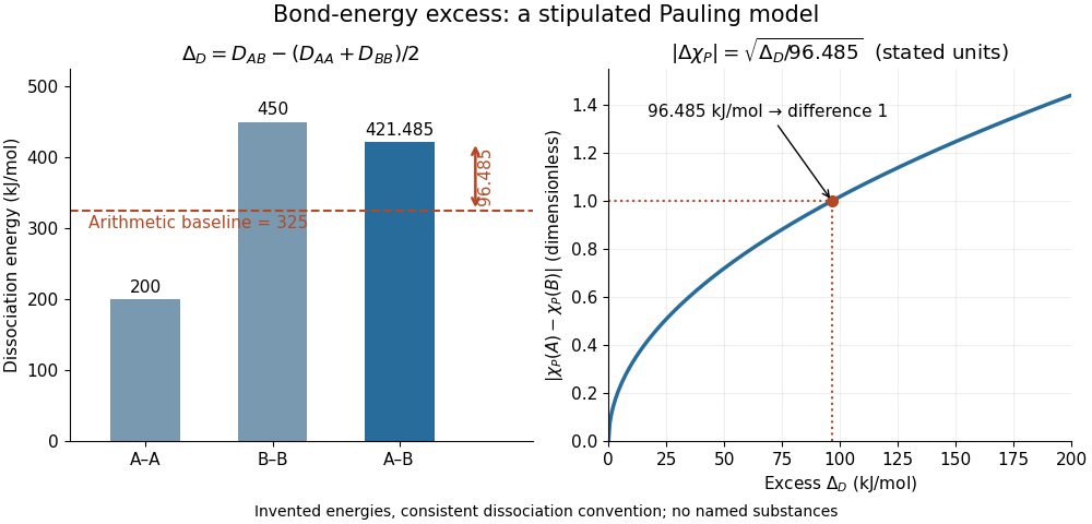
Constructing a Pauling bond-energy excess from stipulated bond-dissociation energies and converting it to a dimensionless electronegativity difference
. Details. Changing the baseline changes the model. For the same stipulated inputs, a geometric mean baseline would be , yielding an excess of and a difference of approximately . It is a different construction, even though both start from the same bond-dissociation energies. State which baseline is used before comparing electronegativity differences.
The arithmetic-baseline Pauling scale also has a useful inverse: a difference of corresponds to an excess of , and a difference of corresponds to . Doubling the electronegativity difference quadruples the modeled excess. Interchanging the endpoint labels changes neither quantity; the square root alone cannot choose the direction of bond polarization.
In The Nature of the Chemical Bond. IV. The Energy of Single Bonds and the Relative Electronegativity of Atoms (printed pp. 3576–3578, Table II and equation (1)), Linus Pauling organized excess energies for chemical bonds into an approximately additive map of their square roots. He also identified a limitation: his H–F map separation of predicted an excess of , exceeding his table's value by . Those are historical values and a historical model discrepancy, not modern recommended inputs.[ref]
The Nature of the Chemical Bond. IV. The Energy of Single Bonds and the Relative Electronegativity of Atoms by Linus Pauling. printed pp. 3576–3578, Table II, equation (1), and paragraph beginning “These coördinates”
A traceless Hermitian matrix in a Hilbert-Schmidt inner product orthonormal basis of the real vector space of traceless Hermitian -by- matrices. One choice uses symmetric and imaginary antisymmetric off-diagonal matrix units, normalized by , and traceless diagonal generators. Together with they form an orthonormal basis of all Hermitian matrices. The coordinates give the Generalized Bloch representation.
For with , take . The spin-down transverse Hamiltonian at momentum label is proportional to , where . It is nonnegative, and gives the displayed zero mode. Since , its exponent has a negative quadratic upper bound at both infinities, proving square integrability for every . The continuously varying momentum label supplies an infinitely degenerate zero-energy space.
The complement of finitely many lines in is path-connected, and any two points can be joined by two line segments. For endpoints outside the lines, exclude the finitely many affine planes through each endpoint and each removed line. Choose a bend point outside all those planes. If either segment met a removed line, the bend point would lie in its associated excluded plane, a contradiction.
The union of with horizontal segments for rational is path-connected. Each point lies either on the vertical spine or on a segment meeting it. A path travels horizontally to the spine, vertically along it, and horizontally to its destination. This contrasts with disconnected rational-slope rays whose common origin has been excluded.
The map for , , is continuous on , since . Its image is the displayed spiral together with its endpoint. The image is compact and path-connected: between images of the explicit path is .
The comoving particle horizon is the particle horizon expressed in comoving coordinates, assuming a finite initial cosmic-time boundary at zero. In a spatially flat FLRW metric, it is the distance a photon could have travelled since that boundary. The corresponding proper distance in cosmology at time is . It differs from the future-directed cosmological event horizon and from the instantaneous comoving Hubble radius.
In a spatially flat FLRW metric, the supremum of the comoving radial distance from which a signal emitted at the initial time can eventually reach a fixed comoving observer is the total conformal time interval. At an intermediate time , this equals its comoving particle horizon plus the comoving radius of its cosmological event horizon, when both integrals converge. This is a visibility bound for emission arbitrarily close to the initial boundary; it does not assert that a transparent universe or a source existed there.
A test particle is an idealized body whose own fields and effect on its environment are negligible. Its motion probes an externally prescribed field. In general relativity, a free massive particle in this limit follows a timelike geodesic, while a free massless particle follows a null geodesic. Nongravitational forces can change either path; appreciable self-gravity requires a more complete treatment.
The partial trace of a positive operator is positive by this sum of nonnegative expectations in an orthonormal basis of the traced factor. Its trace equals the original trace, using the product orthonormal basis. Basis independence follows from , which uniquely determines the reduced operator. Thus reductions of density matrices remain density matrices. For a positive trace-class operator the same argument uses convergent nonnegative basis sums.
A Cauchy problem prescribes a solution and enough of its derivatives on a hypersurface to determine local evolution away from that hypersurface.
A semilinear partial differential equation is linear in its highest-order derivatives, with their coefficients depending only on the independent variables; lower-order terms may depend nonlinearly on the solution and its lower derivatives. A semilinear heat equation such as is an example. This differs from a quasilinear equation, whose highest-order derivative coefficients can depend on the solution or its lower derivatives.
Burgers' equation is the one-dimensional partial differential equationThe term supplies nonlinear transport in a transport equation: the transported value is also its own characteristic speed when . Larger values catch up with smaller values ahead of them, steepening a decreasing profile. The diffusion term opposes this steepening. Positive gives the viscous Burgers equation; setting gives the Inviscid Burgers equation.
This small equation makes three different behaviors accessible in one model: Burgers characteristic breaking from continuous decreasing data, an entropy shock for a downward step, and a rarefaction wave for an upward step. The Burgers Riemann problem with positive flux and the Viscous Burgers travelling shock below give exact examples. These are mathematical calculations with chosen data; the figures contain no experimental measurements.
Unless stated otherwise, take , , constant , no PDE source term, and an initial condition . There are no finite endpoints requiring boundary conditions. Where a profile has different limiting states at , those states are specified explicitly. On a finite interval, boundary conditions become part of the problem: positive diffusion normally requires a condition at each endpoint, whereas the Inviscid Burgers equation requires appropriate inflow transport boundary conditions. With dimensional variables, has units of velocity and of kinematic viscosity; all numerical examples below use dimensionless quantities.
A maximum principle bounds a solution through its boundary or initial data, often forbidding nonconstant solutions from attaining an interior extremum. Weak and strong versions depend on the differential operator and hypotheses. The maximum principle for harmonic functions and its strong counterpart are examples.
Green's identities relate volume integrals involving gradients and Laplacians to boundary values and normal derivatives. They follow from the divergence theorem and include Green's first identity, Green second identity and Green's third identity.
The Kuramoto-Sivashinsky equation combines destabilizing long-wave growth, stabilizing fourth-order diffusion, and nonlinear transport. Its potential form is , with . It arises as a long-wave phase amplitude equation near loss of the Benjamin-Feir stability condition. On a domain of period , the zero solution's Fourier modes grow at rate , .
Pinned article: Introduction to the OurBigBook Project
Welcome to the OurBigBook Project! Our goal is to create the perfect publishing platform for STEM subjects, and get university-level students to write the best free STEM tutorials ever.
Everyone is welcome to create an account and play with the site: ourbigbook.com/go/register. We belive that students themselves can write amazing tutorials, but teachers are welcome too. You can write about anything you want, it doesn't have to be STEM or even educational. Silly test content is very welcome and you won't be penalized in any way. Just keep it legal!
Intro to OurBigBook
. Source. We have two killer features:
- topics: topics group articles by different users with the same title, e.g. here is the topic for the "Fundamental Theorem of Calculus" ourbigbook.com/go/topic/fundamental-theorem-of-calculusArticles of different users are sorted by upvote within each article page. This feature is a bit like:
- a Wikipedia where each user can have their own version of each article
- a Q&A website like Stack Overflow, where multiple people can give their views on a given topic, and the best ones are sorted by upvote. Except you don't need to wait for someone to ask first, and any topic goes, no matter how narrow or broad
This feature makes it possible for readers to find better explanations of any topic created by other writers. And it allows writers to create an explanation in a place that readers might actually find it.
Figure 1. Screenshot of the "Derivative" topic page. View it live at: ourbigbook.com/go/topic/derivativeVideo 2. OurBigBook Web topics demo. Source. - local editing: you can store all your personal knowledge base content locally in a plaintext markup format that can be edited locally and published either:This way you can be sure that even if OurBigBook.com were to go down one day (which we have no plans to do as it is quite cheap to host!), your content will still be perfectly readable as a static site.
- to OurBigBook.com to get awesome multi-user features like topics and likes
- as HTML files to a static website, which you can host yourself for free on many external providers like GitHub Pages, and remain in full control

Figure 2. You can publish local OurBigBook lightweight markup files to either OurBigBook.com or as a static website.
Figure 3. Visual Studio Code extension installation.
Figure 5. . You can also edit articles on the Web editor without installing anything locally. Video 3. Edit locally and publish demo. Source. This shows editing OurBigBook Markup and publishing it using the Visual Studio Code extension. 
- Infinitely deep tables of contents:



All our software is open source and hosted at: github.com/ourbigbook/ourbigbook
Further documentation can be found at: docs.ourbigbook.com
Feel free to reach our to us for any help or suggestions: docs.ourbigbook.com/#contact