Topics (384k) Articles (398k) Users (410) Discussions (242) Comments (383) Files (13k) New article

An optical microscope uses light and optical lens assemblies to reveal small structures, such as the boundaries of biological cells or defects in a manufactured surface. In a compound optical microscope, the microscope objective supplies an enlarged real image; the microscope eyepiece makes that intermediate microscope image subtend a larger viewing angle. The transverse magnification of the first stage and the angular magnification of the second answer different questions.[ref]
2.8 Microscopes and Telescopes. University Physics Volume 3, §2.8 Microscopes, image formation and Eqs. 2.35–2.37
Consider an original ideal finite-conjugate microscope in air, with both optical lens assemblies treated as converging thin lens elements in the paraxial approximation. Choose objective focal length and object distance . The thin lens equation and signed transverse magnification givePlace a microscope eyepiece of focal length a further beyond the intermediate microscope image. The objective-to-eyepiece separation is therefore . Each object point then supplies a parallel outgoing bundle of light rays, appropriate to a relaxed eye focused at infinity. Define the unaided reference as the same object viewed at distance ; this is a rating convention, not a universal property of eyesight. The eyepiece angular magnification and total signed angular magnification areFor instance, a hypothetical object height becomes at the intermediate microscope image. The signed viewing angles are approximately with the instrument and unaided. Their ratio is : enlarged and inverted. These are stipulated model dimensions, not measurements or specifications of a modern commercial optical microscope.
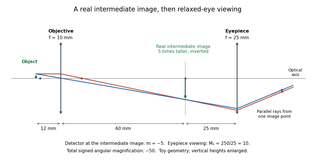
The attraction of an optical microscope is that seeing can become measuring: a stage micrometer supplies a known object-space length, and microscope scale calibration converts an image readout into a specimen length. This also separates a large-looking image from a trustworthy size estimate. Meanwhile, diffraction-limited resolution depends on numerical aperture and wavelength; empty magnification enlarges an existing blur without revealing additional structure.
A convective chimney is a localized deeply mixed region formed when surface buoyancy loss overcomes ocean density stratification. Small plumes, compensating flow, rotation and lateral exchange maintain its structure; it need not be a permanently uniform descending column. Brine rejection can increase its surface density forcing. A fresh summer cap can isolate a deep homogeneous core until winter forcing renews contact with the surface, so a surviving core need not imply continuous active convection.
A polar body is a small product of the unequal divisions of oogenesis. The divisions separate chromosomes while retaining most cytoplasm in the developing ovum. Producing several chromosome-containing products therefore need not mean producing several equivalent eggs.
In the standard human account, the first polar body follows the first meiotic division; completion of the second division produces another. Their formation illustrates the difference between chromosome segregation and equal partition of cellular resources.[ref]
If a buoyant plume of diameter supplies oil at volume rate to an ice floe moving at speed , the plume sweeps area per unit time. Retaining a layer of depth over that area would require volume rate , so conservation of mass gives the painted fraction . Discontinuous painting starts when . This estimate assumes all arriving oil is retained and a constant track width equal to the plume diameter; the plume's circular cross-sectional area does not enter the swept-area rate.
Two eye-specific afferent populations compete under Hebbian learning and synaptic normalization. In a simplified symmetric two-eye model, the eye-difference mode evolves with a linear operator containing . Dominant spatial modes can produce alternating eye preference, while saturation sets finite contrast. The interaction width, arbor constraints and correlation structure influence the column scale. This is a mechanistic hypothesis whose predictions can be tested, not a unique inference from the existence of columns.
An isophote is a contour of equal surface brightness in an astronomical image. Deviations from fitted ellipses encode additional information about a galaxy's projected stellar structure.
Surface brightness is received flux per unit solid angle on the sky. It describes the brightness of an extended source independently of a particular aperture's area. An isophote is a contour of constant surface brightness; central surface brightness sets the available photons for resolved galaxy spectroscopy.
Angular resolution describes the smallest angular separation or structure an observation can distinguish. A physical scale at distance subtends approximately radians when . Resolving a black-hole sphere of influence therefore involves distance as well as its physical radius, and useful kinematics also require adequate surface brightness.
For a nearby Euclidean survey with limiting flux , a galaxy of luminosity is detectable out to . Its accessible volume is therefore proportional to . With a Schechter function , counts per logarithmic interval are proportional to and peak at when . This selection suppresses faint objects relative to a volume-limited census; finite survey boundaries and cosmological evolution modify the simple law.
The Arnowitt-Deser-Misner formalism expresses general relativity as constrained Hamiltonian evolution of a spatial metric and its conjugate momentum after a 3+1 decomposition of spacetime. Lapse and shift enforce the Hamiltonian and momentum constraints. For an asymptotically flat spacetime its boundary Hamiltonian gives the Arnowitt-Deser-Misner energy.
An iterative method approximates a solution by repeatedly updating an initial guess. In numerical linear algebra, a stationary iterative method for a linear system uses a fixed iteration map; other iterations can change their update rule or search space at each step.
The QR algorithm computes eigenvalues through repeated QR decompositions and similarity updates. Shifted and unshifted forms have different convergence rates; the unshifted QR algorithm uses a zero shift at every step.
A collocation method chooses an approximate solution from a finite-dimensional trial space and forces the residual of a differential equation to vanish at selected nodes. Collocation Runge-Kutta methods apply this principle to polynomial approximations on each time step.
The midpoint method advances an ordinary differential equation using a derivative evaluated at a temporal midpoint. Its explicit form predicts that midpoint from the initial derivative, while the implicit midpoint rule solves for the derivative at the mean of the endpoint states.
A linear multistep method approximates an ordinary differential equation using values retained from several time levels. On a uniform grid , its constant-coefficient form isThe linearity is in the way values and derivatives are combined; the vector field itself can be nonlinear. The method is explicit when and implicit when the new value appears inside through . An implicit update requires a suitable algebraic solve, in addition to a formal recurrence.[ref]
A special stability problem for linear multistep methods by Germund Dahlquist. §1, equation 1.2 and explicit/implicit distinction, printed p. 27
The two-step Adams-Bashforth method, for example, uses . It reuses the preceding derivative rather than calculating several new Runge-Kutta stages within one step. A -step recurrence needs starting values, often supplied by a Runge-Kutta method of compatible accuracy.
Consistency controls the defect on a smooth exact solution; zero-stability controls the amplification of starting and local errors. Both are required by the Dahlquist equivalence theorem for convergence under its regularity assumptions. Changing the step sizes generally requires changing the coefficients and revisiting stability; uniform-grid coefficients cannot simply be reused at arbitrary time spacings.
The Thomas algorithm is Gaussian elimination specialized to a tridiagonal matrix: each row couples an unknown only to its immediate neighbours. Eliminating one unknown changes just the next diagonal entry and right-hand side. Provided all pivot elements are nonzero, a forward sweep followed by back substitution solves an -unknown linear system in time and storage, using Big O notation. Treating the same entries as a full matrix wastes the zeros: classical dense LU factorization and solve costs grow cubically for factorization and quadratically for storage.
A concrete reason to care is the Dirichlet Poisson solution by tridiagonal elimination: a three-point finite difference for the second derivative couples adjacent points on a mesh, producing precisely this tridiagonal matrix. The same structure occurs in one-dimensional Crank-Nicolson method calculations. NPTEL's archived Lecture 13 introduces the Thomas algorithm from that time-stepping problem and labels the procedure “Thomas algorithm (1949)”.[ref]
Thomas algorithm (NPTEL Lecture 13). Lecture 13, Thomas algorithm: opening historical attribution and Crank Nicolson motivation
Interpolation constructs a function agreeing exactly with prescribed values at sample points. The resulting function is an interpolant. Choosing a family determines how missing values are filled: polynomial interpolation selects a polynomial, while linear interpolation joins adjacent samples by straight segments. The McShane extension theorem instead permits any Lipschitz function with a specified bound and provides envelopes controlling all allowed choices.
Error control selects discretization parameters and checks approximations against requested accuracy. Local error estimators, absolute and relative error tolerances and an adaptive step-size controller provide practical local control. Propagation of defects determines the global error, while stiffness, roundoff error and algebraic-solve accuracy impose additional limits.
For an ordinary differential equation, the practical loop is to propose a step, form a local error estimator, scale it by absolute and relative error tolerances, and accept or retry before choosing the next step. An embedded Runge-Kutta pair supplies two endpoints from shared Runge-Kutta stages, making this extra accuracy check inexpensive. The Euler-Heun embedded pair below exposes the distinction between the accepted formula's order of a numerical method and the estimator's step exponent; its Adaptive Euler-Heun integration of exponential growth shows accepted local tests alongside accumulated global error.
Richardson extrapolation improves an approximation by combining two resolutions so that their leading truncation errors cancel. The useful surprise is that the size of that leading error need not be known: its scaling under refinement is enough. This lets an existing finite difference method or quadrature rule produce a more accurate answer from two runs, without first deriving a new method from scratch.
Suppose approximates a fixed limit as the positive resolution parameter tends to zero, with an asymptotic expansionHere is known, is independent of , and denotes Big O notation. The same asymptotic expansion, with the same , must describe both and . Nested grids make it natural to reuse samples, although nesting itself does not establish this error model. Define the linear combinationThe weights sum to one, preserving , while . Thus Richardson extrapolation gives : the next available term in the asymptotic expansion determines the improved order. Justin Solomon's numerical analysis text develops this cancellation for finite differences and applies it to numerical integration.[ref]
https://people.csail.mit.edu/jsolomon/share/book/numerical_book.pdf. Justin Solomon, Numerical Algorithms, §14.3.3 and Exercise 14.9
Geometrically, regard the approximation as a function of . Its first two terms are a straight line . The two computed points lie at positive ; extending the line through them to gives . This is why the operation is extrapolation: it estimates a value outside the sampled parameter interval. The remaining curvature corresponds to the uncancelled terms of the asymptotic expansion.
Worked example: a centered derivative of sine. For the smooth function , the exact derivative at is . The centered difference quotient, a central finite difference, isThe Taylor series of sine gives the signed truncation errorThus , and . Halving divides the leading truncation error by four. Combining the two centered difference quotients with Richardson extrapolation givesIndeed, the coefficient becomes ; the coefficient vanishes. This is the even-power case of Richardson extrapolation discussed in Persson's authored lecture notes.[ref]
https://persson.berkeley.edu/math128a/lecture_notes/math128a_lecture_notes_chapter_4.html. Per-Olof Persson, Math 128A, Chapter 4, §§4.1–4.2
For and , the actual computations areThe absolute error drops from about for to for , an improvement by roughly a factor of 498. Refining again gives , whose absolute error is about . The refined truncation errors decrease by nearly four for and nearly sixteen for , reflecting their second and fourth orders.
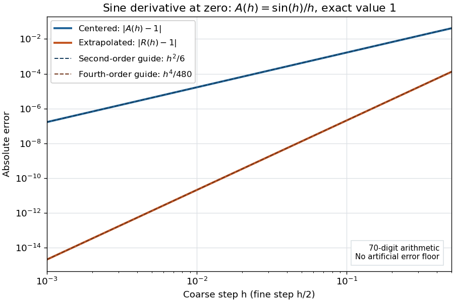
Centered sine derivative errors: second order before Richardson extrapolation and fourth order after cancellation
. Source. Details. The logarithmic scale on each axis turns power laws into straight lines. The dashed reference curves are and , the magnitudes of the leading truncation errors. The plotted errors are computed with 70-digit decimal arithmetic, rather than clipped to a display floor; this isolates the asymptotic expansion from roundoff error.
Worked example: integrating an exponential. Approximate the definite integral of the exponential function on :For numerical integration, the composite trapezoidal rule adds the areas of trapezoids between successive samples; this is the quadrature use of the endpoint average that also occurs in the ODE trapezoidal rule. On equal intervals, with , defineSumming the geometric series gives . Expanding the exponential function near zero yieldsThe leading truncation error again has , . On the uniform nested grids with and intervals, Richardson extrapolation therefore givesThis linear combination is exactly composite Simpson's rule on the finer grid, whose spacing is . On each coarse panel, an old endpoint receives weight and the new midpoint weight ; shared old endpoints receive weight . These are the usual Simpson's rule weights multiplied by . The equivalence is explained directly in LeMesurier's university notes.[ref]
https://lemesurierb.people.charleston.edu/elementary-numerical-analysis-python/notebooks/definite-integrals-3-simpson-richardson.html. Brenton LeMesurier, MATH 375, §19.1: The Basic Simpson's Rule by Richardson Extrapolation
For two coarse panels and four fine panels,The absolute errors are about , and , respectively. Reusing the fine-grid samples makes Richardson extrapolation especially attractive here: the resulting Simpson's rule needs no samples beyond those already used by .
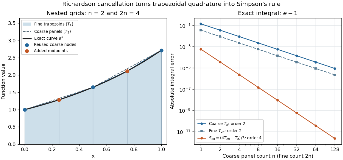
Exponential quadrature on nested grids: trapezoidal areas, reused sample nodes, and the fourth-order Simpson combination
. Source. Details. When the improvement is justified. Richardson extrapolation requires the stated asymptotic expansion and the correct positive . If the actual leading exponent is , its coefficient after combination is , so the leading truncation error generally remains. Merely knowing does not supply a common coefficient or a higher-order remainder. A discontinuity of a function, a singular endpoint, or unrelated changes between grids can invalidate the assumed asymptotic expansion; refinement alone does not guarantee improvement for every numerical problem.
Roundoff error and errors in the sampled values survive the cancellation of truncation error. If the coarse and fine values have absolute perturbations bounded by , the perturbation in is bounded by ; for this is . In floating-point arithmetic, a centered difference quotient can also amplify sample errors through division by , so an indefinitely smaller need not be more accurate. Persson's notes describe this balance between truncation error and roundoff error.[ref]
https://persson.berkeley.edu/math128a/lecture_notes/math128a_lecture_notes_chapter_4.html. Per-Olof Persson, Math 128A, Chapter 4, §4.1: Roundoff Error Instability
The same cancellation idea appears in step-doubling error estimation. For an order- one-step method for an ordinary differential equation, two half steps each contribute local truncation error of order , so their accumulated leading local error has ratio to one full step. This explains the denominator there; the appropriate exponent follows from that local error model, rather than automatically from a generic use of Richardson extrapolation.
Pinned article: Introduction to the OurBigBook Project
Welcome to the OurBigBook Project! Our goal is to create the perfect publishing platform for STEM subjects, and get university-level students to write the best free STEM tutorials ever.
Everyone is welcome to create an account and play with the site: ourbigbook.com/go/register. We belive that students themselves can write amazing tutorials, but teachers are welcome too. You can write about anything you want, it doesn't have to be STEM or even educational. Silly test content is very welcome and you won't be penalized in any way. Just keep it legal!
Intro to OurBigBook
. Source. We have two killer features:
- topics: topics group articles by different users with the same title, e.g. here is the topic for the "Fundamental Theorem of Calculus" ourbigbook.com/go/topic/fundamental-theorem-of-calculusArticles of different users are sorted by upvote within each article page. This feature is a bit like:
- a Wikipedia where each user can have their own version of each article
- a Q&A website like Stack Overflow, where multiple people can give their views on a given topic, and the best ones are sorted by upvote. Except you don't need to wait for someone to ask first, and any topic goes, no matter how narrow or broad
This feature makes it possible for readers to find better explanations of any topic created by other writers. And it allows writers to create an explanation in a place that readers might actually find it.
Figure 1. Screenshot of the "Derivative" topic page. View it live at: ourbigbook.com/go/topic/derivativeVideo 2. OurBigBook Web topics demo. Source. - local editing: you can store all your personal knowledge base content locally in a plaintext markup format that can be edited locally and published either:This way you can be sure that even if OurBigBook.com were to go down one day (which we have no plans to do as it is quite cheap to host!), your content will still be perfectly readable as a static site.
- to OurBigBook.com to get awesome multi-user features like topics and likes
- as HTML files to a static website, which you can host yourself for free on many external providers like GitHub Pages, and remain in full control

Figure 2. You can publish local OurBigBook lightweight markup files to either OurBigBook.com or as a static website.
Figure 3. Visual Studio Code extension installation.
Figure 5. . You can also edit articles on the Web editor without installing anything locally. Video 3. Edit locally and publish demo. Source. This shows editing OurBigBook Markup and publishing it using the Visual Studio Code extension. 
- Infinitely deep tables of contents:




All our software is open source and hosted at: github.com/ourbigbook/ourbigbook
Further documentation can be found at: docs.ourbigbook.com
Feel free to reach our to us for any help or suggestions: docs.ourbigbook.com/#contact