Topics (384k) Articles (398k) Users (410) Discussions (242) Comments (383) Files (13k) New article
The parallactic angle is the angle between the great circles from an observed direction toward the celestial pole and toward the zenith. Its change gives sky rotation in pupil-stabilized observations.
An RLC circuit combines electrical resistance , inductance , and capacitance . The capacitor stores energy in its electric field; the inductor stores energy in its magnetic field. Their exchange can produce an oscillation, while Joule heating removes energy. A series RLC circuit gives a particularly clear example: changing turns ringing into a direct return to equilibrium, and changing or tunes a resonance.
These circuits connect two useful viewpoints. In time, they describe how stored energy is released after switching. In frequency, they select a range of signals: the resonant series RLC response explains radio tuning and simple filters. The same mathematics describes a damped harmonic oscillator, so insight about mechanical ringing transfers directly to an electrical circuit. [ref]
https://www.feynmanlectures.caltech.edu/I_23.html#Ch23-S3. Feynman lectures, I.23.3: electrical and mechanical resonance
; [ref]https://www.feynmanlectures.caltech.edu/II_22.html#Ch22-S7. Feynman lectures, II.22.7: frequency filters
.Gas drag is a drag force on a solid body due to its motion relative to surrounding gas. With aerodynamic stopping time , the linear approximation gives .
The drag coefficient measures a drag force against a specified scale of force. Let be the body's velocity relative to the distant, undisturbed fluid, and let be its relative speed. For fluid density , drag force magnitude and reference area , defineThe drag coefficient is a dimensionless quantity: the denominator has units of force. The reference area must be reported with it. For a sphere of radius , the usual choice is the frontal area . Choosing its entire surface area instead divides the reported drag coefficient by four for the same physical drag force. Comparing coefficients without comparing their reference areas can therefore be misleading. [ref]
https://www1.grc.nasa.gov/beginners-guide-to-aeronautics/drag-coefficient/. NASA Glenn Research Center, Drag Coefficient, definition and Determining Value for Drag Coefficient
For a rigid sphere in steady flow through an unbounded Newtonian fluid with constant dynamic viscosity , incompressible flow and the no-slip boundary condition, the creeping-flow limit requires the diameter-based particle Reynolds number . The Stokes drag law gives . Substitution into the definition with gives the short derivationThus the drag coefficient is neither necessarily constant nor bounded above by one. The formula containing still describes linear drag here, because the drag coefficient varies as . The relation is the leading small-Reynolds number approximation, not a measured curve valid at every Reynolds number. [ref]
https://farside.ph.utexas.edu/teaching/336L/Fluid/node142.html. Richard Fitzpatrick, Axisymmetric Stokes Flow Around a Solid Sphere, equations 10.126 and 10.129
For a worked example, stipulate dynamic viscosity , density , radius and relative speed . Within the stated Stokes drag law assumptions,Doubling the relative speed with all other parameters fixed gives and : the predicted drag force doubles to . Falsely holding the drag coefficient at would instead quadruple the drag force. Both particle Reynolds numbers remain small, so the comparison is within the creeping-flow approximation.
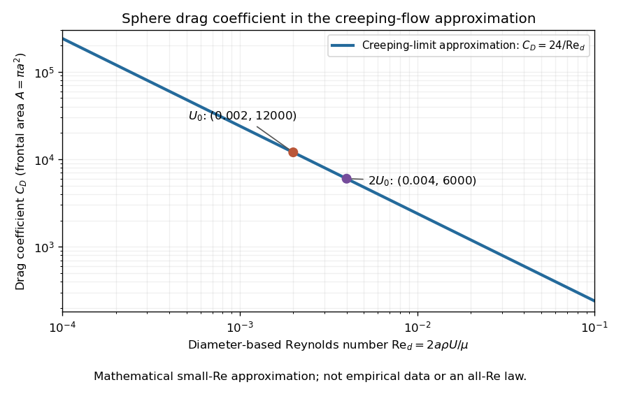
The useful idea is to separate the force scale from the dependence on geometry and flow conditions. A drag coefficient can help compare experiments, but changing Reynolds number can change the coefficient itself; NASA Glenn explicitly stresses matching the relevant flow conditions. The elegant cancellation above also exposes a common mistake: a drag coefficient definition does not by itself impose a quadratic drag law.
Linear drag opposes the velocity relative to the surrounding medium with magnitude proportional to its speed, where . Its power is , so it dissipates kinetic energy. Under a constant external force, the resulting linear ordinary differential equation relaxes exponentially on the time scale .
Paley–Wiener theorems relate spatial support or decay to analytic continuation and growth of the Fourier transform. Different versions apply to square-integrable functions or to distributions. The Paley–Wiener–Schwartz theorem is the distributional version.
The support of a distribution is the complement of the largest open set on which its pairing vanishes for every supported test function. A partition of unity shows that the union of such open sets still has this vanishing property. For example, the Dirac delta distribution and all its derivatives have support .
The combined operation of charge conjugation and parity symmetry in quantum field theory. A weak interaction can preserve this symmetry while violating each constituent separately.
A second-order difference equation determines the next member of a sequence from its two preceding values, for example . Two initial values are generally needed. Although the state is written with one scalar sequence, the update becomes a first-order discrete dynamical system on pairs:
Two directed acyclic graphs are Markov equivalent when they encode the same D-separations for all disjoint sets of vertices. They consequently impose the same global Markov property for a directed acyclic graph, although their causal interpretations can differ.
A differential operator is in divergence form when its highest derivatives occur inside a divergence, for example or . This form makes integration by parts express the operator through a lower-order bilinear form and boundary flux.
The formal transpose is defined by the bilinear integration by parts identity for test functions. For , it is ; unlike the Hermitian adjoint operator, it does not conjugate coefficients.
Differentiability is the existence of a derivative at a point. For maps between finite-dimensional normed vector spaces, the existence of a Fréchet derivative requires a single linear map approximating the increment with error . Merely having partial derivatives need not provide this approximation; continuous partial derivatives on a neighbourhood do suffice.
Accelerated contraction has and , so the magnitude increases. Since , it corresponds to a first Hubble slow-roll parameter .
A stationary point is nonisolated if every neighbourhood contains other stationary points. For a twice differentiable function, a regular smooth curve of stationary points through a point forces its Hessian matrix to annihilate the curve's nonzero tangent: differentiate the vanishing gradient along the curve. Thus the Hessian matrix has a zero eigenvalue there, but that alone need not determine whether the point is a local minimum or local maximum.
A real-valued function , with , has a local maximum at if some satisfiesOnly a neighbourhood within the domain of a function is compared. Equality is allowed; a strict local maximum requires for every other point in that neighbourhood. A constant function therefore has a local maximum and a local minimum at every input, with neither strict. This is a local form of an extremum of a real-valued function.
For , zero is a strict local maximum because when . It is not a global maximum: values far away grow without bound. This distinction makes a local maximum useful for describing a nearby peak without claiming that it is the highest value anywhere.
Negating the function exchanges local maxima and local minima, including their strict versions. At a smooth interior local maximum, the critical point argument forces zero gradient; for a function twice continuously differentiable nearby, its Hessian matrix is negative semidefinite. These necessary conditions alone do not establish a local maximum.
The endpoint of a gas-liquid phase coexistence curve, where the distinct liquid and gas states merge. For a smooth fluid equation of state, the critical isotherm has at this point; this thermodynamic meaning differs from a stationary critical point of an arbitrary function.
A simple random walk on a cycle graph of vertices has expected value of its cover time equal to , from any starting vertex. Lift the walk to the integers using the same increments. Its contiguous visited interval covers all residues precisely when it reaches length . Sum the expected time to expand a random-walk range, , using linearity of expectation; no independence of expansion times is needed.
Bernoulli coupling by a shared uniform random variable by  Codex 0 Created 2026-10-05 Updated 2026-10-14
A noninteracting perfect fluid in general relativity has , so . If energy is transferred between species, source terms appear and only their sum vanishes. The Friedmann equation still involves the sum of all component stress tensors because all components share one spacetime metric.
Pinned article: Introduction to the OurBigBook Project
Welcome to the OurBigBook Project! Our goal is to create the perfect publishing platform for STEM subjects, and get university-level students to write the best free STEM tutorials ever.
Everyone is welcome to create an account and play with the site: ourbigbook.com/go/register. We belive that students themselves can write amazing tutorials, but teachers are welcome too. You can write about anything you want, it doesn't have to be STEM or even educational. Silly test content is very welcome and you won't be penalized in any way. Just keep it legal!
Intro to OurBigBook
. Source. We have two killer features:
- topics: topics group articles by different users with the same title, e.g. here is the topic for the "Fundamental Theorem of Calculus" ourbigbook.com/go/topic/fundamental-theorem-of-calculusArticles of different users are sorted by upvote within each article page. This feature is a bit like:
- a Wikipedia where each user can have their own version of each article
- a Q&A website like Stack Overflow, where multiple people can give their views on a given topic, and the best ones are sorted by upvote. Except you don't need to wait for someone to ask first, and any topic goes, no matter how narrow or broad
This feature makes it possible for readers to find better explanations of any topic created by other writers. And it allows writers to create an explanation in a place that readers might actually find it.
Figure 1. Screenshot of the "Derivative" topic page. View it live at: ourbigbook.com/go/topic/derivativeVideo 2. OurBigBook Web topics demo. Source. - local editing: you can store all your personal knowledge base content locally in a plaintext markup format that can be edited locally and published either:This way you can be sure that even if OurBigBook.com were to go down one day (which we have no plans to do as it is quite cheap to host!), your content will still be perfectly readable as a static site.
- to OurBigBook.com to get awesome multi-user features like topics and likes
- as HTML files to a static website, which you can host yourself for free on many external providers like GitHub Pages, and remain in full control

Figure 2. You can publish local OurBigBook lightweight markup files to either OurBigBook.com or as a static website.
Figure 3. Visual Studio Code extension installation.
Figure 5. . You can also edit articles on the Web editor without installing anything locally. Video 3. Edit locally and publish demo. Source. This shows editing OurBigBook Markup and publishing it using the Visual Studio Code extension. 
- Infinitely deep tables of contents:



All our software is open source and hosted at: github.com/ourbigbook/ourbigbook
Further documentation can be found at: docs.ourbigbook.com
Feel free to reach our to us for any help or suggestions: docs.ourbigbook.com/#contact