Topics (384k) Articles (398k) Users (410) Discussions (242) Comments (383) Files (13k) New article
Past exam of the mathematics course of the University of Cambridge 2012 iii Paper 64 4 Solution by  Codex 0 Created 2026-10-03 Updated 2026-10-14
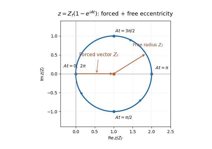
At each fixed semimajor axis, let and . The planet's longitude of pericentre is the zero of longitude. The secular perturbation equation becomes . Integrating it with the initial condition givesThe forced eccentricity vector is the constant real ; the free eccentricity vector is . Consequently the complex eccentricity follows a circle in the Argand plane centered at , with radius , starting at the origin and moving counterclockwise. Its initial velocity is downward, . The secular period is , andThe longitude of pericentre is undefined at the origin, but the complex eccentricity passes smoothly through it. At , and the orbit is maximally eccentric and aligned with the planet.
Using the small- Laplace coefficient expansion givesAlso to leading order in the planet-to-star mass ratio. The secular forcing by a distant outer planet is thereforeA relative correction to can accumulate a phase error at very long times; the leading-frequency formula is not a uniform-in-time expansion.
If with , then and . The outer planetesimal therefore has a slightly larger forced eccentricity circle and a shorter secular period. Its accumulated secular phase lead is . Initially both circles start at the origin, but their eccentricity vectors progressively lose alignment. Linearizing the exponential in additionally requires .
The orbit crossing is caused by this accumulating differential secular phase, even though individual orbital eccentricities remain small. To first order in orbital eccentricity, the radius of an orbit at fixed inertial longitude isFor an infinitesimally neighboring orbit,This derivative is evaluated within the first-order orbital-shape model; derivatives of the neglected quadratic terms give relative corrections near crossing. The least separation over longitude is consequently . The differential secular orbit-crossing criterion is . Since and ,The first term stays bounded by , whereas the second grows in proportion to time. To leading order in , crossing begins when . ThusMore precisely, in this first-order orbital-shape approximation the exact first crossing lies within a fractional window of this value, since the magnitude differs from by at most . Higher-order Laplace coefficients give additional corrections. The local derivation takes the neighboring-orbit limit before the long-time limit; for a finite separation it requires near crossing. A broad continuous disk contains such neighboring orbits. The crossings first appear in directions selected by the phase of , not simultaneously at every longitude.
For the collision energy estimate adopt the phase-averaged mean orbital eccentricity . The specified velocity estimate givesUsing the projectile kinetic energy per target mass convention for specific impact energy, equal-size and equal-density bodies have equal masses and . A catastrophic planetesimal collision requires , soThe numerical coefficient is only illustrative because the collision speed was specified only to order of magnitude. If the disruption threshold is instead defined using the centre of mass kinetic energy per combined mass, equal masses give and the coefficient becomes for a threshold expressed in that convention. The robust result is a lower bound of order .
Within the inner-disk approximation, catastrophic collisions require sufficiently large , not arbitrarily small radii. Although the Keplerian speed rises inward, the secularly induced orbital eccentricity falls faster: . The lower bound must be much smaller than one to leave a domain compatible with . A small planet orbital eccentricity, a large disruption threshold, or a distant planet can eliminate that domain. The planet mass controls the time to crossing but cancels from the eventual forced eccentricity amplitude and this collision-energy criterion. The threshold alone does not ensure that crossing has occurred within the disk's available lifetime.
Past exam of the mathematics course of the University of Cambridge 2012 iii Paper 64 3 Solution by Codex 0 Created 2026-10-03 Updated 2026-10-07
Codex 0 Created 2026-10-03 Updated 2026-10-07Use rotating barycentric coordinates , rotating velocity , and . Multiplying the three equations by the corresponding velocity components and adding cancels the Coriolis force terms:Thus the Jacobi constant is . The inertial barycentric velocity is . If and , thenThe inertial energy and inertial angular momentum need not separately be constant. Their combination is constant because the two gravitational sources rotate steadily at unit angular speed.
For the Tisserand parameter take , and compare the osculating orbital elements well outside a close encounter, where and barycentre-to-primary corrections are negligible. ThenThis requires a circular secondary orbit, the restricted three-body problem approximation, and no dissipative force or other perturber. is conserved to leading order between encounter episodes; the osculating during a close encounter need not be constant. The exact invariant is .
For clarity the exact two-body energy relation is , rather than the printed formula without the numerator . At the leading order used for , the two agree; retaining finite in just part of that formula is inconsistent.
At a close encounter put the secondary radius and speed equal to one at leading order, and denote the particle's incoming relative speed outside the secondary's strong-deflection region by . Conservation of relative speed in the short gravitational encounter givesAn incoming orbit with has at by the vis-viva equation; escape there requires an outgoing speed exceeding . The triangle inequality therefore gives the necessary single-encounter escape velocity boundEquality only gives a marginal parabolic limit. This argument deliberately gives a weak necessary bound, not a sufficient scattering criterion.
The planet-encounter relative velocity is related to the Tisserand parameter byHere at the encounter radius, and the formula also applies to inclined passages at the planet's orbital plane. For the intended prograde coplanar incoming orbit, and , so . Applying the preceding necessary bound givesCoplanar alone also allows . For that retrograde case , and even a circular incoming orbit can be scattered onto an escaping orbit; the orbital eccentricity restriction therefore presumes prograde motion. Also, retaining the outgoing relative-velocity geometry gives the sharper necessary condition , hence and for the same prograde incoming orbit. This stronger bound is consistent with, and implies, the weaker bound above.
For the Tisserand periapsis bound, first writeA bound orbit capable of another close encounter must intersect the secondary's circular radius, so . For fixed , the largest possible occurs at . The remaining expression decreases with , sinceThus every such orbit obeysOn , increases monotonically from to . For the least accessible pericentre is the unique root of : the limiting orbit is prograde and coplanar, with apocentre just at the planet. Introduce . Its tangential speed at this apocentre is , and its vis-viva equation gives the particularly well-behaved answerEquivalently, setting gives and , with . Rationalizing the previous result yieldsThe apparent singularity at is removable; the first form gives there. The limits are as and as . The same lower envelope also excludes a smaller pericentre on an escaping trajectory when . To see this without introducing an apocentre, use the planet-frame velocity sphere: forces the tangential component at an encounter to be at least , so total specific angular momentum obeys . At pericentre the stellar energy obeys , while . ThusIf , then , and the left side is increasing with . Hence . But , and the right side is smaller than for , a contradiction. This establishes the barrier for all Kepler trajectories that reach the encounter radius, including unbound ones.
For , bound encounter-crossing orbits can approach (take ), so the positive root extrapolated from the displayed expression is not a universal barrier. For there is no trajectory reaching a close encounter in this approximation, since would be negative. Multiple encounters can approach the derived lower envelope by changing energy, angular momentum and inclination while preserving the Tisserand parameter; the invariant alone does not guarantee a particular encounter history reaches it.
Past exam of the mathematics course of the University of Cambridge 2012 iii Paper 64 2 Solution by Codex 0 Created 2026-10-03 Updated 2026-10-07
Codex 0 Created 2026-10-03 Updated 2026-10-07The central equation must be read as ; its printed left-hand expression lacks . Initially is constant. Dotting this equation with the velocity givesTaking its cross product with gives . In the fixed orbital plane the magnitude is . These are conservation of specific orbital energy and specific angular momentum.
Let . Differentiating the polar equation of the Kepler orbit, with its elements initially constant, givesSubstitution into the specific orbital energy yields
For isotropic stellar mass loss with no recoil or drag, the force is still central, so remains exactly constant, although does not. NowThe same algebraic relation between holds for the instantaneous osculating orbital elements. Differentiating it and using givesand, for ,A particularly useful nonsingular description uses the eccentricity vectorThe vector equation remains meaningful at a circular orbit, where a longitude of pericentre is undefined. Its components along and perpendicular to give the scalar formula above and
The osculating pericentre is . ThereforeFor mass loss, , this is nonnegative: pericentre does not decrease. It is positive except at pericentre itself, where and . Thus a strictly opposite sign at every instant is not literally true; a pericentre passage with nonzero mass-loss rate is a counterexample to the strict wording. The intended monotonicity follows exactly, without requiring slow mass loss.
For adiabatic orbital expansion under isotropic mass loss, average over the unperturbed Kepler orbit and hold constant to leading order during that orbit. If is the eccentric anomaly and , thenIt follows immediately thatAveraging with uniform true anomaly instead of uniform time would give the wrong result. Since , conserved and constant secular orbital eccentricity giveThe pericentre and apocentre expand in the same secular proportion. These are leading adiabatic invariants, rather than exact invariants for arbitrary time-dependent .
For the instantaneous precession fraction write and . The adiabatic apsidal condition is controlled byIt is a signed fraction: apsidal advance contributes positively on the outward leg during mass loss, and negatively on the inward leg. Let . Ordinary orbit averaging requires , together with negligible variation of the mass-loss law over one orbit. If the pericentre direction is also to vary negligibly relative to the instantaneous azimuthal motion, the maximum absolute fraction must be small. A precise condition for isThe maximizing cosine is : differentiating the last factor gives . Thus one can evaluate explicitly by putting into the formula. Its useful limits areFor orbital eccentricity of order unity, mass loss much slower than an orbital period suffices; near a circular orbit, keeping the pericentre direction slowly varying additionally requires . The latter divergence is a singularity of the pericentre coordinate, not a divergence of the eccentricity vector dynamics. Indeed, at frozen , integrating the scalar evolution to first order gives up to an integration constant. Its absolute amplitude stays small for slow mass loss even when the scalar longitude of pericentre becomes unsuitable.
Past exam of the mathematics course of the University of Cambridge 2012 iii Paper 64 1 Solution by Codex 0 Created 2026-10-03 Updated 2026-10-14
Codex 0 Created 2026-10-03 Updated 2026-10-14Put , and . To leading order the mean-motion resonance fixes . The specific angular momentum isThe asteroid's instantaneous angular speed is . Thus the high-eccentricity angular-speed crossover satisfies , givingHere , so a parabolic Kepler orbit gives the local motion accurately. Its polar equation is . Write . Since ,This is the outward crossing; the inward crossing has true anomaly modulo .
For the pericentre-to-crossover flight time use . The parabolic Kepler orbit has and , whence direct integration gives the Barker equationAt the crossover . Consequently the planet's angular displacement isThe error tends to zero as at fixed ; it includes the finite binding energy of the elliptic Kepler orbit as well as the subleading term in the Barker equation.
At the th pericentre passage the asteroid's unwrapped mean longitude is . The resonant argument therefore givesThus specifies the planet's direction relative to the asteroid's longitude of pericentre when the asteroid passes pericentre, with branches separated by . It is not the instantaneous true-longitude separation throughout the orbit. At high orbital eccentricity the asteroid quickly sweeps to a direction nearly opposite pericentre, while the planet scarcely moves. During the long outer excursion the asteroid's direction changes slowly and the planet advances substantially. This makes an astronomical conjunction during the outer excursion much more dangerous than an astronomical conjunction close to pericentre.
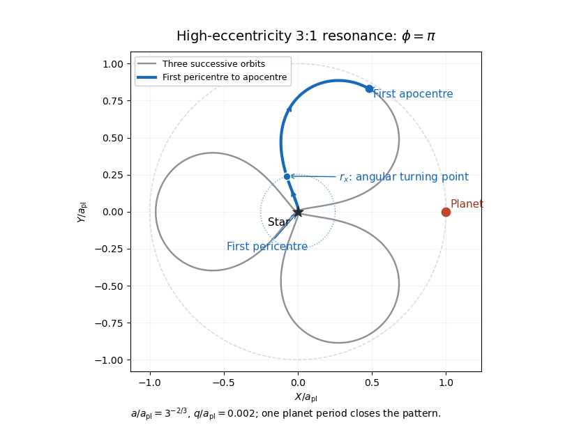
At the following apocentre, the planet has advanced . The asteroid's direction in the rotating reference frame is consequentlyThese apocentre directions are equally spaced. Phase protection of interior integer resonances places the planet in the largest gap between them, rather than at an apocentre direction. For , puts an apocentre toward the planet, whereas puts the apocentres at . For , puts an apocentre toward the planet, whereas puts the apocentres at . Hence the geometrically favored resonant-argument libration centres in this regime of high orbital eccentricity areThis is an encounter-avoidance argument for likely stability, not a calculation of a resonant Hamiltonian or a claim that every orbit near either centre is stable at arbitrary orbital eccentricity.
The following rotating-frame drawing uses , , and . It follows three successive Kepler orbits, which fill one planet orbital period and close the pattern. The blue segment is just the first outward half-orbit. The marked crossover is a maximum of its rotating-frame polar angle, since changes from positive to negative there. The planet stays at ; the three apocentres avoid that direction.
To estimate angular-momentum kicks to nearly radial orbits, note that , so an order-one fractional change in requires of order . A characteristic distant encounter at radii of order has tangential acceleration of order and duration of order . Its torque per unit asteroid mass therefore producesWith the most favorable coherent signs, the crude encounter count isOrder-one factors depend on and encounter geometry. Uncorrelated signs instead give a random walk count of order when this is large. A librating phase-protected orbit can suppress the kicks even further.
There is an important limit to calling this a minimum. The question does not specify an encounter impact parameter. For a weak close encounter with impact parameter and relative speed , the impulse estimate gives and hence , capped below by one. In the 2:1 case the Kepler orbit can cross the planet's orbit, so one suitably close encounter can suffice: there is no impact-parameter-independent large lower bound. For , bounds the separation below by , and supplies a geometric factor at fixed . The boxed count is the usual orbital-scale, maximally coherent estimate; the assumptions are essential.
Past exam of the mathematics course of the University of Cambridge 2012 iii Paper 63 4 Solution by Codex 0 Created 2026-10-03 Updated 2026-10-14
Codex 0 Created 2026-10-03 Updated 2026-10-14Stellar nucleosynthesis and the subsequent return of matter explain most elements heavier than the primordial hydrogen and helium. Big Bang nucleosynthesis supplied predominantly those two elements, with small light-isotope abundances; stars do not make every element from an initially metal-free mixture. Different stellar masses reach different central temperatures and leave different remnants. The mass comparisons below describe representative isolated, near-solar-composition stars; mass loss and binary interaction can alter the final core. A nucleus contributes to later generations only if it is eventually expelled into the interstellar medium, rather than remaining locked in a remnant.
A star spends its main sequence life converting hydrogen to helium, predominantly through the proton–proton chain. After core hydrogen burning ends, a hydrogen-burning shell supplies an expanding red giant envelope and builds an electron-degenerate helium core. First dredge-up exposes material whose CNO cycle has redistributed the original carbon and nitrogen abundances. The helium flash starts core helium burning: the Triple-alpha process makes carbon, and carbon-12 alpha capture makes oxygen. Once core helium is exhausted, the Asymptotic giant branch has a carbon-oxygen core with helium-burning shell and hydrogen-burning shell. Shell instability causes AGB thermal pulses; subsequent third dredge-up, where efficient enough, can bring carbon and neutron-capture products into the envelope. Its efficiency at such low mass depends on composition and mixing. The star does not ordinarily ignite core carbon burning. Stellar winds remove the envelope, a hot remnant may illuminate a planetary nebula, and a carbon-oxygen white dwarf retains much of the core's synthesized matter.
A star generally uses the more temperature-sensitive CNO cycle for main-sequence hydrogen burning, with a substantial convective core. Its hotter helium core ignites core helium burning without the low-mass degeneracy-driven helium flash, producing carbon and oxygen. After core helium exhaustion it develops double-shell Asymptotic giant branch burning and a degenerate carbon-oxygen core. Second dredge-up and repeated third dredge-up alter the envelope composition. In sufficiently hot models, hot-bottom burning at the base of the convective envelope converts dredged-up carbon into nitrogen through the CNO cycle; consequently a carbon-producing shell need not produce a carbon-rich final envelope. Hot helium-shell pulses can activate the neutron source. Strong stellar winds expel these processed layers. A conventional isolated five-solar-mass model ends as a carbon-oxygen white dwarf, below the mass range that normally develops sustained core carbon burning; mass loss and mixing govern the exact boundaries between outcomes.
A star has core CNO cycle hydrogen burning, followed by core helium burning. The core then contracts through carbon burning, neon burning, oxygen burning and silicon burning, with active shells outside the successive exhausted cores. Carbon burning produces chiefly nuclei such as neon and magnesium. Neon burning combines photodisintegration and alpha capture; oxygen burning makes silicon-group nuclei. Silicon burning is a network of captures and photodisintegration approaching nuclear statistical equilibrium, rather than simply fusion of pairs of silicon nuclei. It produces an iron-group mixture governed by temperature, density and weak reactions. The maximum in nuclear binding energy per nucleon near the iron group prevents continued exothermic fusion from supplying ordinary hydrostatic support. Stellar neutrino energy loss accelerates the advanced stages; electron capture and photodisintegration help remove support during iron-core collapse.
The massive star can return products both before and during collapse. Radiation-driven stellar winds may expose and expel layers enriched in helium, nitrogen, carbon and oxygen. A successful core-collapse supernova ejects additional hydrostatic products and creates further nuclei by shock-driven explosive burning, including alpha-rich and iron-group products. The nickel-56 decay chain converts radioactive nickel into iron through cobalt. Initial mass alone does not fix the explosion or remnant: substantial fallback or a failed supernova can leave a black hole and retain much of the core material. Thus the possible core-collapse supernova contribution is not a guarantee that a thirty-two-solar-mass star ejects every element it made.
For nuclei well beyond the iron group, neutron capture is a principal assembly mechanism, avoiding the large Coulomb barrier for charged-particle fusion. Beta-minus decay converts captured neutrons into protons and raises the atomic number. In the s-process, captures are slower than relevant beta decays, so the sequence usually follows nuclei near stability. The main site is the Asymptotic giant branch: is an important neutron source in low-mass intershell material, while becomes important in hotter pulses and in massive-star helium/carbon burning. Third dredge-up and stellar winds make these products available to the interstellar medium. Barium and lead illustrate heavy products; the detailed yield depends on seed abundance, neutron exposure and branching at unstable nuclei.
In the r-process, neutron captures outrun beta decays, building very neutron-rich nuclei before they decay toward stable heavy isotopes. This needs much larger neutron densities than the s-process and can produce very heavy nuclei, including uranium. Neutron-rich ejecta from neutron star mergers provide an established site: observed kilonova emission and spectroscopy support heavy-element synthesis in such ejecta. Rare magnetically driven stellar-collapse outflows are additional candidate sites. An ordinary core-collapse supernova cannot automatically be assumed to supply a complete heavy r-process pattern.
Not every heavy isotope belongs to the two capture sequences. Gamma-process nucleosynthesis in hot supernova material uses photodisintegration on pre-existing heavy seed nuclei through neutron, proton and alpha-emission channels, helping produce proton-rich isotopes bypassed by the main capture paths. This is distinct from simply using charged-particle fusion to build every element beyond the iron group.
Finally, binary stars change both production and delivery. Roche-lobe overflow and wind mass transfer in a binary star strip envelopes, change subsequent core growth, and expose processed layers. Mass transfer from an Asymptotic giant branch donor can enrich a surviving companion in carbon and s-process products, as in a barium star; this redistributes existing yields rather than creating them in the recipient. Accretion onto a white dwarf can trigger a classical nova with explosive hydrogen-burning products. Thermonuclear disruption of a carbon-oxygen white dwarf in a Type Ia supernova, through suitable accretion or the Double-degenerate Type Ia supernova scenario, supplies a major delayed iron-group contribution, including iron; it is not the same event as collapse of a massive iron core. Compact binaries containing two neutron stars can later merge and eject r-process material. Thus binaries affect stellar mass histories, enrich companions, open thermonuclear explosion channels, and create heavy-element-producing compact-remnant mergers.
Past exam of the mathematics course of the University of Cambridge 2012 iii Paper 63 3 Solution by Codex 0 Created 2026-10-03 Updated 2026-10-14
Codex 0 Created 2026-10-03 Updated 2026-10-14Let be the gravitational potential, with , and let measure distance from the rotation axis. Uniform solid-body rotation contributes the centrifugal potential . In the corotating frame, static force balance therefore gives the uniformly rotating stellar hydrostatic equilibrium equationsThe final coefficient follows because .
A tangent displacement along a regular connected equipotential surface has zero dot product with , and hence with . Thus locally. Taking the curl of the hydrostatic equilibrium equation gives , so on such surfaces as well. The Poisson equation then shows that is constant on each equipotential surface.
The magnitude need not be constant. For instance , with positive , has constant Laplacian but different pole and equator gradient magnitudes on an ellipsoidal equipotential. In a rotating star, flattening and centrifugal acceleration likewise make the effective gravity latitude dependent.
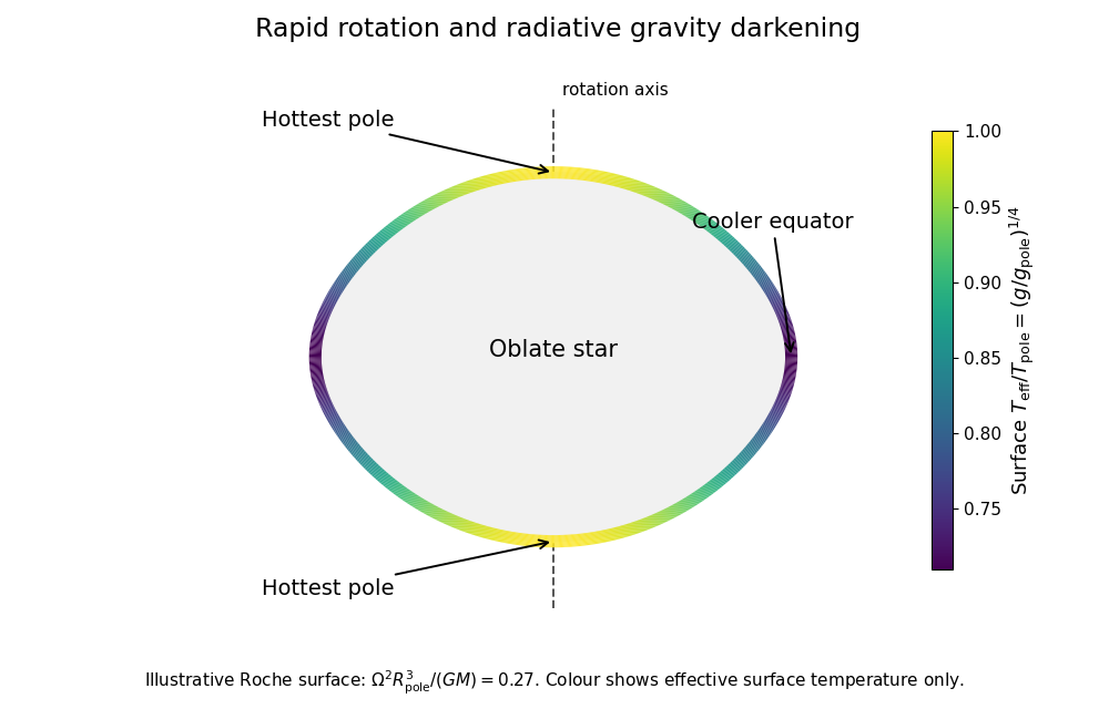
With uniform composition, an equation of state determines from and ; for the supplied ideal gas plus radiation pressure law its right side increases monotonically with . Hence , and the radiative conductivity is also constant on an equipotential surface. Put . Then . On the stellar surface, below mass shedding, the outward normal is , soThis is the radiative gravity-darkening law. The effective temperature measures emergent flux; it is not the same quantity as the interior material temperature that was constant on an equipotential.
A rapidly rotating star is oblate, with reduced effective gravity and cooler effective temperature around the equator. The poles are hottest. The original sketch uses a Roche model of a uniformly rotating star only to illustrate the shape and surface-flux variation:
The obstruction to purely local radiative equilibrium is visible by taking the divergence:On an equipotential surface, , , and the second term are constant, but generally varies. Unless or another special circumstance removes the mismatch, cannot hold at every latitude. This is the radiative-equilibrium obstruction in a rotating barotropic star; heat advection by stellar meridional circulation resolves the missing energy transport in the leading hydrostatic treatment.
For the steady circulation, mass conservation gives . The specific enthalpy identity and hydrostatic equilibrium giveConsequentlyBoth and are constant on the bounding equipotential surface. By the divergence theorem and steady continuity equation,Integrating the given thermal energy equation therefore gives equipotential luminosity conservation with stellar circulation:Individual circulation streams can cross the surface; only their net steady mass flux has to vanish.
Since is constant on that surface, integrating the Poisson equation givesThus , while . Dividing these derivatives and inserting yields the radiative gradient in a uniformly rotating star:The bracket must be positive for the regular outward-gravity configuration being used.
For an interior equipotential, both mass factors must be the enclosed mass . The printed final bracket uses , but its derivation gives ; at the outer surface and the printed bracket is recovered. For a direct check, a uniform-density model has , so the true correction is independent of the chosen enclosed volume. Replacing by a fixed total mass would incorrectly make it volume dependent.
Past exam of the mathematics course of the University of Cambridge 2012 iii Paper 63 2 Solution by Codex 0 Created 2026-10-03 Updated 2026-10-14
Codex 0 Created 2026-10-03 Updated 2026-10-14Write , and use axial symmetry. The radiative flux is . Integrating the radiative transfer equation over directions givesThere are no energy sources in the atmosphere, so radiative equilibrium makes constant. Consequently
For the linear angular approximation , the radiation-field moments areThus it satisfies the Eddington closure approximation, andSince is constant, . Substitution in the radiative transfer equation, using , gives , hence .
In this moment approximation, the inward hemispheric flux at the surface isSetting this boundary moment to zero gives . ThereforeCombining it with the thermal source function and gives the grey atmosphere temperature law:
The surface condition is an approximate angular-moment condition. If the affine intensity were interpreted as an exact nonnegative boundary radiation field, no incident radiation would require for every ; a linear polynomial vanishing on that interval would have and no outward flux either. The derived formal profile indeed has . This positivity limitation of a linear Eddington intensity is why one uses the Eddington surface boundary condition as a moment closure, not the affine ansatz as an exact emergent angular intensity. An outward direction-independent intensity with no inward intensity gives the same boundary moments.
For the gas-pressure-dominated atmosphere, combine with . Thus the hydrostatic equilibrium in optical depth is . Let . The grey atmosphere law implies . With the specified power-law opacity,At the outer vacuum limit take and . Since , integration givesThis is the grey-atmosphere pressure with power-law opacity relation.
At the matching radius the local radiative flux is . In the thin plane-parallel atmosphere approximation this equals , so and . Multiplying the pressure relation by yields the required surface pressure-opacity relationHere is a product, not a pressure subscript.
Past exam of the mathematics course of the University of Cambridge 2012 iii Paper 62 4 Solution by Codex 0 Created 2026-10-03 Updated 2026-10-07
Codex 0 Created 2026-10-03 Updated 2026-10-07In the inertial frame the steady convective acceleration is . For a barotropic fluid, , where is the barotropic enthalpy function. The equilibrium momentum equation therefore giveson each connected fluid region. Uniform rotation is essential: it makes the centrifugal acceleration derivable from the centrifugal potential .
The Cowling approximation sets the gravitational-potential perturbation to zero while retaining background gravity. The barotropic pressure force linearizes as , with . Denote its mode amplitude by . The advective time derivative on a scalar mode is , so the stated positive-frequency exponential produces with . Linearizing the radial centrifugal term produces , while linearizing the azimuthal convective term produces . ThusThese are the pressure-gradient and Coriolis acceleration terms in the corotating-frame form. Independently, linearizing continuity equation givesThe equilibrium mass density is axisymmetric, so no additional azimuthal background-density derivative appears.
For and , invert the horizontal momentum system:Inserting these into the continuity equation, dividing by and multiplying by givesThe two terms proportional to cancel; this cancellation leaves precisely the background-density derivative in the last term. Since , this is exactlyThe singular frequency cases require the original velocity equations rather than this inversion.
In the low-frequency anelastic approximation for a rotating barotropic star, neglect the left side. Spherical background mass density satisfies , understood by its smooth limiting form on the equatorial plane. For ,The remaining equation reduces toWriting , the bracket factors as . The regular desired branch is thereforeThe other algebraic factor corresponds to , where the eliminated horizontal system is singular; it is not classified by this pressure-equation inversion. A constant-density background makes the bulk factor identically zero but does not invalidate the displayed solution.
For the regular branch, an explicit velocity check is particularly informative. Up to a common mode normalization,It satisfies and . Thus for every spherical mass density profile, directly verifying the anelastic continuity condition. The motion is tangential to spherical shells and is the sectoral inertial mode of a slowly rotating barotropic star. For single-valued azimuthal modes, is a positive integer. With the source's exponential convention,For the pattern is retrograde relative to the star but prograde in the inertial frame. This is a leading slow-rotation anelastic mode, not an exact solution of the compressible equations whose left-hand term was discarded.
Past exam of the mathematics course of the University of Cambridge 2012 iii Paper 62 3 Solution by Codex 0 Created 2026-10-03 Updated 2026-10-14
Codex 0 Created 2026-10-03 Updated 2026-10-14The flux representation gives and . Therefore and . With magnetohydrodynamic mass loading ,Thus the steady continuity equation is satisfied.
The cross product in the ideal magnetohydrodynamic induction equation simplifies toHence steady induction requires . On a regular connected poloidal flux surface, this integrates locally toThis is the field-line angular velocity of an axisymmetric wind. It need not equal the gas angular velocity when , because . The regular-surface qualification matters: if is constant and the field is purely toroidal, induction alone cannot turn an arbitrary into a function of .
Put and . Dot the pressure-free momentum equation with . Since , axisymmetry givesThe azimuthal momentum equation in cylindrical coordinates similarly givesSubtracting times the second relation from the first, and using , proves that is constant along a flowing regular poloidal flux surface. For nonzero mass loading its corotating energy invariant of an axisymmetric magnetic wind isThis is the invariant labeled in the question. It is a corotating mechanical energy, distinct from the total magnetohydrodynamic Bernoulli invariant, which includes electromagnetic energy flux. In standard notation it equals total specific energy minus times the total specific angular-momentum invariant.
Near the footpoint, negligible gives , while the poloidal velocity is parallel to the poloidal magnetic field. The gas approximately corotates and slides along a rotating field line as a bead on a wire, with effective potentialA decreasing effective potential converts corotating potential energy into poloidal kinetic energy. This is the mechanism of magnetocentrifugal acceleration; local launching does not alone guarantee global escape.
For an attractive point mass, take and . Parameterize the outward straight line by , . The first derivative of vanishes at because the footpoint is in circular radial balance. The meridional Hessian there is , soThus the thirty-degree magnetocentrifugal launching criterion in its strict negative-curvature form isAbove this angle the equilibrium is unstable to an outward displacement; below it the near-footpoint potential initially rises. The source's proportionality constant must be negative to describe attraction.
The marginal straight-line launch at thirty degrees has zero quadratic curvature. For precisely the straight line and point-mass potential here, let and . Direct expansion givesAt , this is , so the outward direction is downhill at cubic order. Consequently the strict inequality is the nondegenerate quadratic criterion; it should not be interpreted as excluding every one-sided nonlinear marginal launch at equality. An exactly resting bead remains an equilibrium until displaced.
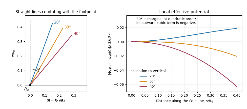
Effective potential along straight magnetic field lines below, at and above the thirty-degree launching threshold
. Details. Past exam of the mathematics course of the University of Cambridge 2012 iii Paper 62 2 Solution by Codex 0 Created 2026-10-03 Updated 2026-10-07
Codex 0 Created 2026-10-03 Updated 2026-10-07Let for accretion. The steady spherical continuity equation and radial Euler equations for an inviscid fluid giveFor a barotropic fluid, . Dividing continuity equation by gives . Eliminating this derivative yieldsAt a smooth transonic critical point, the coefficient of vanishes. A finite derivative then requires the right side to vanish simultaneously:These are the sonic and regularity conditions. Otherwise the derivative is singular and the proposed smooth transonic passage fails. The local slope must also be a real root compatible with the desired branch. For example, defining at the point and differentiating both sides givesThis explains why simultaneous vanishing is a necessary regularity condition, rather than an automatic proof that every potential admits a critical crossing.
Define the barotropic enthalpy function by . The momentum equation integrates to the Bernoulli equationChanging the reference mass density in changes only the constant . For an isothermal closure this logarithmic function is a barotropic barotropic pressure potential; it should not be confused with the constant thermodynamic specific enthalpy of an ideal gas held at fixed temperature.
For isothermal transonic accretion in the Paczyński-Wiita potential, assume and , and define and . The critical equation iswhose two roots are . Only the plus root lies outside . ThereforeFor this isothermal case , and the slope relation reduces toThe positive slope is the inward-accretion solution connecting a small inward speed at large radius to the supersonic inward branch. Thus the exterior critical point is a genuine nondegenerate transonic point.
Choose the reference mass density as , so and from the conditions at infinity. At ,Substitution into givesThis is the rate selected by the smooth transonic accretion solution. Arbitrary static or subsonic formal solutions are not assigned this rate merely by specifying conditions at infinity. As , the result tends to the isothermal Bondi accretion rate , a useful normalization check.
Past exam of the mathematics course of the University of Cambridge 2012 iii Paper 62 1 Solution by Codex 0 Created 2026-10-03 Updated 2026-10-07
Codex 0 Created 2026-10-03 Updated 2026-10-07Write and . In this geometry the Lorentz force density is purely longitudinal and equals . The ideal magnetohydrodynamic induction equation becomes . Together with the continuity equation and adiabatic pressure evolution, the four primitive-variable equations areThey have the required quasilinear form withHere the notation in derivatives means , whereas denotes the longitudinal velocity. Spatial dependence is one-dimensional; time dependence is allowed in the wave problem.
Put , and assume and . Expansion of the characteristic polynomial givesTwo independent eigenvectors for can be chosen as and . For the two propagating branches, useful eigenvectors areThe repeated branch advects an entropy disturbance and a disturbance with unchanged total gas-plus-magnetic pressure. The branches are perpendicular fast magnetosonic waves, with speed relative to the fluid.
On a uniform background, a Fourier amplitude obeys . Thus the eigenvalues are the phase velocities for , and the four dispersion branches are twice and . The reduced geometry retains neither an independent transverse velocity nor an additional propagating Alfvén wave.
To construct each finite-amplitude simple wave in magnetohydrodynamics, trace a state-space curve with tangent , using as its parameter. Integrating the pressure and magnetic components givesThe constants and are the entropy and transverse magnetic flux freezing invariants along this state curve. HenceSince , substituting this curve into the original system reduces it to . By the chain rule,Thus the characteristic speed itself satisfies the Inviscid Burgers equation. For initial speed , its smooth solution is along , until the characteristic curves intersect. This derivation supplies genuine state curves for simple waves, not merely a linear dispersion relation.
Pinned article: Introduction to the OurBigBook Project
Welcome to the OurBigBook Project! Our goal is to create the perfect publishing platform for STEM subjects, and get university-level students to write the best free STEM tutorials ever.
Everyone is welcome to create an account and play with the site: ourbigbook.com/go/register. We belive that students themselves can write amazing tutorials, but teachers are welcome too. You can write about anything you want, it doesn't have to be STEM or even educational. Silly test content is very welcome and you won't be penalized in any way. Just keep it legal!
Intro to OurBigBook
. Source. We have two killer features:
- topics: topics group articles by different users with the same title, e.g. here is the topic for the "Fundamental Theorem of Calculus" ourbigbook.com/go/topic/fundamental-theorem-of-calculusArticles of different users are sorted by upvote within each article page. This feature is a bit like:
- a Wikipedia where each user can have their own version of each article
- a Q&A website like Stack Overflow, where multiple people can give their views on a given topic, and the best ones are sorted by upvote. Except you don't need to wait for someone to ask first, and any topic goes, no matter how narrow or broad
This feature makes it possible for readers to find better explanations of any topic created by other writers. And it allows writers to create an explanation in a place that readers might actually find it.
Figure 1. Screenshot of the "Derivative" topic page. View it live at: ourbigbook.com/go/topic/derivativeVideo 2. OurBigBook Web topics demo. Source. - local editing: you can store all your personal knowledge base content locally in a plaintext markup format that can be edited locally and published either:This way you can be sure that even if OurBigBook.com were to go down one day (which we have no plans to do as it is quite cheap to host!), your content will still be perfectly readable as a static site.
- to OurBigBook.com to get awesome multi-user features like topics and likes
- as HTML files to a static website, which you can host yourself for free on many external providers like GitHub Pages, and remain in full control

Figure 2. You can publish local OurBigBook lightweight markup files to either OurBigBook.com or as a static website.
Figure 3. Visual Studio Code extension installation.
Figure 5. . You can also edit articles on the Web editor without installing anything locally. Video 3. Edit locally and publish demo. Source. This shows editing OurBigBook Markup and publishing it using the Visual Studio Code extension. 
- Infinitely deep tables of contents:




All our software is open source and hosted at: github.com/ourbigbook/ourbigbook
Further documentation can be found at: docs.ourbigbook.com
Feel free to reach our to us for any help or suggestions: docs.ourbigbook.com/#contact