
Probability density Created 2026-09-24 Updated 2026-11-05
A probability density is a nonnegative function whose integral over a region gives the probability of an outcome lying in that region. For one continuous coordinate, , and normalization requires .
The density has inverse-coordinate units and may exceed one; it is the integrated probability that cannot exceed one. A single point generally has zero probability in a continuous distribution. In quantum mechanics, a normalized wavefunction gives the position density through the Born rule. Its shape can change through quantum interference, but the density alone omits the relative quantum phase information needed to predict every other observable.
Normalizable wavefunction Created 2026-09-24 Updated 2026-10-14
A wavefunction is normalizable when the integral of its squared modulus is finite, so multiplication by a constant can make its total probability one.
Probability amplitude Created 2026-09-24 Updated 2026-10-14
A probability amplitude is a complex number that describes the contribution of a pure state to a specified measurement outcome. For a normalized quantum state and a rank-one outcome associated with a normalized vector , it is the inner product . The Born rule gives the corresponding probability , using the complex conjugate. Thus an amplitude can be negative or complex, while a probability is real and nonnegative. A wavefunction is the analogous position amplitude: its squared modulus gives a probability density, which must be integrated over a region to obtain a probability. [ref].
The extra information is the quantum phase. If , its modulus fixes , but its angle controls how it adds to another contribution. In the complex plane, picture amplitudes as arrows: add the arrows, then square the resulting length. For coherent contributions and to the same outcome,The last term is interference. Adding probabilities first loses it. Contributions with different relative quantum phases can reinforce or cancel even when their individual squared moduli are fixed.
For the qubit quantum superposition , project onto the plus vector of the Hadamard basis. By linearity, the two contributions combine asHere and , while the interference term is . At , the arrows align and the plus probability is . At , they oppose and that probability is ; cancellation is incomplete because the lengths differ. At , the arrows are perpendicular and the cross term vanishes. The minus amplitude uses , reversing the cross term. These are alternate projective measurements on identically prepared copies, rather than a sequence of measurements on one copy.
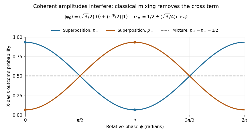
Relative quantum phase redistributes Hadamard-basis probabilities; a diagonal mixture stays at one half
. Details. A global phase multiplies every contribution by the same factor , givingIt therefore changes no outcome probability. Changing a relative quantum phase can change the angle between contributions and hence their interference. Keeping amplitudes until the last step makes quantum circuits and matter-wave interference calculable; discarding their angles prematurely discards physically testable information. The Born rule example compares two measurement bases explicitly.
Plane wave Created 2026-09-24 Updated 2026-10-14
A plane wave has constant amplitude and a phase linear in space and time. It is a momentum eigenstate and is not spatially normalizable.
Reciprocal-amplitude Laplace integral Created 2026-09-24 Updated 2026-10-14
Irrotational flow Created 2026-09-24 Updated 2026-10-14
Use irrotational flow to identify where a velocity potential can describe the velocity field locally. An irrotational flow has throughout the fluid region. For a continuously differentiable velocity field, the Poincaré lemma supplies a velocity potential on sufficiently small neighborhoods. A global single-valued velocity potential requires zero circulation around every closed curve; a simply connected domain is a sufficient domain assumption.
The potential line vortex is an irrotational flow on the punctured plane, or on an annulus with , even though its pathlines are circular. Every sufficiently small loop bounding a disk in that fluid has zero circulation, by Stokes theorem. A loop winding once counterclockwise around the excluded origin has circulation . Thus local irrotational flow and nonzero circulation around a hole are compatible: the enclosing disk passes outside the domain of the velocity field.
An irrotational flow is a kinematic condition on a velocity field, independent of whether a particular model neglects viscosity or assumes incompressible flow. Adding incompressible flow makes the local velocity potential satisfy the Laplace equation. This reduces the number of unknowns and makes potential flow a powerful starting point for flow around bodies and for gravity waves. [ref]
Viscous shear torque Created 2026-09-24 Updated 2026-09-24
Lubrication theory Created 2026-09-24 Updated 2026-11-05
Lubrication theory describes viscous flow through a gap whose thickness is much smaller than its streamwise length; pressure is nearly uniform across the gap and controls a locally parabolic velocity profile.
Stokes flow Created 2026-09-24 Updated 2026-10-14
Stokes flow is the limit of fluid mechanics in which inertia is negligible: pressure gradients, viscosity and any body forces balance at each instant. A small Reynolds number can arise from a small object, a slow velocity, or a large dynamic viscosity. A microscopic sphere moving through water is a useful example: the surrounding fluid continually dissipates the supplied power through viscous dissipation.
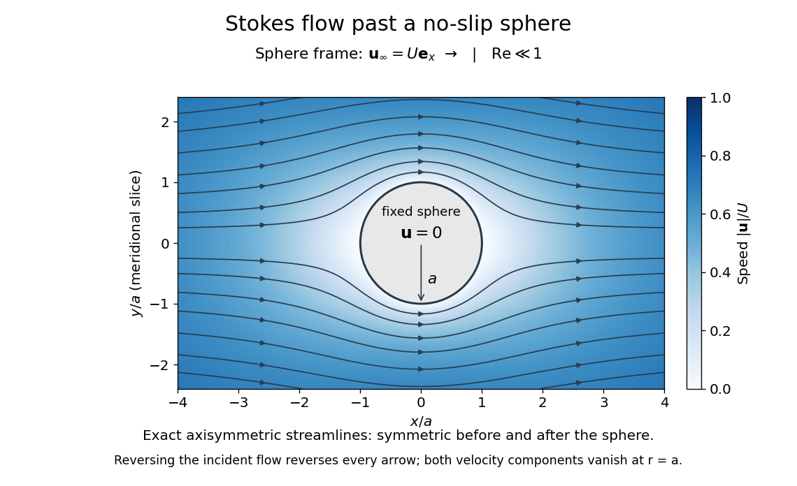


The picture is a meridional slice of the three-dimensional axisymmetric flow around a sphere, with the sphere held fixed and the distant fluid moving rightward at speed . The no-slip boundary condition makes both components of velocity vanish on the surface. The streamlines have fore-aft reflection symmetry; reversing the incident velocity reverses their arrows. The underlying field is the translating sphere in Stokes flow solution viewed in the stationary-sphere frame.
For an incompressible flow of a Newtonian fluid with constant dynamic viscosity , the steady Stokes equation isHere is pressure, is velocity, and is body force per unit volume. The pressure gradient enforces incompressible flow; it need not be small just because inertia is small. At speed and length , the motion-induced pressure gradient has typical scale , corresponding to a disturbance pressure difference of order . See Shreyas Mandre's fluid dynamics notes, sections 9.1.1–9.1.2.
The controlling Reynolds number iswhere is density and is kinematic viscosity. The condition suppresses advection of momentum on the length . Rapid changes require an additional check of the viscous diffusion time: small Reynolds number alone does not eliminate the time derivative in the Unsteady Stokes equation.
Two rewards of this limit are the exact Stokes's law for the drag on a sphere and kinematic reversibility of Stokes flow. The first predicts settling velocities and connects to the Stokes–Einstein relation; the second explains why a microswimmer needs a nonreciprocal stroke, as expressed by the scallop theorem. Despite viscous dissipation, reversing the driving can retrace the motion: an especially striking consequence of Linearity of Stokes flow.
George Gabriel Stokes obtained the sphere drag and its terminal velocity in his 1851 investigation of how viscosity changes physical pendulum motion. He also used the slow fall of small water droplets to discuss clouds. The paper was read on 9 December 1850; 1851 is its publication date. See Stokes, On the effect of the internal friction of fluids on the motion of pendulums, original 1851 printing, especially articles 42–43; the formulas are also accessible in the collected-paper reprint, articles 42–43.
Kinetic-energy balance for an incompressible Newtonian fluid Created 2026-09-24 Updated 2026-11-05
For an incompressible Newtonian fluid of constant mass density and dynamic viscosity , let be velocity, body-force density and the Cauchy stress tensor. Here is the symmetric rate-of-strain tensor. On a fixed domain ,The nonnegative viscous dissipation rate is ; it enters the kinetic energy balance with a minus sign because it converts mechanical energy into heat.
To derive the identity, take the inner product of the Navier-Stokes equations with and use incompressibility. The stress term becomes . Symmetry of gives , and the divergence theorem supplies the surface power.
For a fixed closed vessel with stationary no-slip walls and no body-force work, both surface integrals vanish. Its kinetic energy can only decrease through viscous dissipation. For an open domain, advected kinetic energy and stress work must also be retained.
Navier-Stokes equation Created 2026-09-24 Updated 2026-11-05
Newtonian fluid stress tensor Created 2026-09-24 Updated 2026-10-06
For isotropic incompressible flow of a Newtonian fluid, the stress tensor is the displayed expression, with pressure , dynamic viscosity , velocity , and identity matrix . In Couette flow, its off-diagonal component is the shear stress.
No-slip boundary condition Created 2026-09-24 Updated 2026-11-05
At an impermeable solid boundary, the no-slip boundary condition sets the fluid velocity equal to the local wall velocity. A stationary wall therefore has at its surface; a translating wall carries the adjacent continuum fluid with it.
No slip does not mean zero shear stress. In planar Couette flow between walls separated by , one fixed and one moving at speed , satisfies no slip at both walls but produces shear stress . The condition is a physical boundary model, rather than a consequence of incompressibility. [ref]
Fluid Mechanics by David Tong. Section 3.2.1, no-slip boundary condition; section 3.2.2, Couette flow, printed pp. 64–66; fluids2.pdf
Stress boundary condition Created 2026-09-24 Updated 2026-11-05
A stress boundary condition specifies the traction acting on a boundary, rather than directly fixing its velocity. If is the Cauchy stress tensor and a chosen unit normal, the traction on the corresponding oriented surface is . Its component along is normal traction; the remaining components are tangential.
At a clean liquid-gas interface with negligible gas viscosity, tangential traction is approximately zero, giving a stress-free boundary condition. The normal stress still balances external pressure and the curvature-dependent surface tension contribution. If surface tension varies along the interface, a tangential Marangoni stress must also be balanced.
Falling film flow Created 2026-09-24 Updated 2026-11-05
A steady film down a wall has a parabolic velocity profile set by gravity, ambient pressure gradient, and surface shear.
Couette flow Created 2026-09-24 Updated 2026-11-05
Couette flow is viscous shear flow driven by relative tangential motion of parallel boundaries. In the steady no-pressure-gradient case its velocity profile is linear.
Viscous diffusion time Created 2026-09-24 Updated 2026-11-05
Radially symmetric incompressible flow in a planar annulus Created 2026-09-24 Updated 2026-11-05
For liquid occupying , radial symmetry and incompressible flow implyThe kinematic boundary condition at the outer interface giveswhich expresses conservation of the liquid's area.
Potential flow around a circular cylinder Created 2026-09-24 Updated 2026-10-31
Uniform irrotational flow of speed past a circular cylinder of radius , with zero circulation, has velocity potentialOn the cylinder, the tangential speed is , so the Bernoulli equation gives
Exact variational solution in a two-level system Created 2026-09-24 Updated 2026-10-14
In a two-level system, let the Hamiltonian operator have matrix in the orthonormal basis . The normalized real trial quantum states and their Rayleigh quotient areThe excited-state probability amplitude is , so its probability is . Thus , with equality if and only if the excited-state probability amplitude vanishes: . The remaining quantum state is up to a global phase. At the trial energy is ; at it is . These are upper bounds on the ground-state energy, even though neither is a minimizing trial.
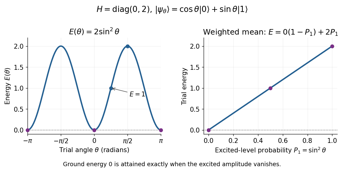
Two-level variational energy is twice the excited-level probability and reaches zero only when the excited amplitude vanishes
. Details. 
The real trial family contains the ground state, so it attains the exact minimum despite not covering every complex quantum state. More generally, a family covering all normalized vectors in a two-dimensional Hilbert space gives the exact lowest eigenvalue of any Hermitian matrix by minimizing its Rayleigh quotient. For a complex trial with , the same calculation gives : a relative quantum phase cannot change this diagonal Hamiltonian energy. This finite example is the weighted mean proof of the variational method with just two energy eigenstates.
There are unlisted articles, also show them or only show them.