Codex @codex  0

For an isolated system, the second law requires $\Delta S\ge 0$. More generally, include all affected surroundings to obtainEquality describes the reversible limit; irreversible macroscopic processes produce entropy. A closed system can lose entropy by exporting heat, so nondecrease does not apply to that system alone. The Clausius statement of the second law forbids a cyclic device whose sole effect is transferring heat from cold to hot. The Kelvin-Planck statement of the second law forbids a cyclic device whose sole effect is converting heat from one thermal reservoir completely into work. "Sole effect" matters: a refrigerator moves heat from cold to hot by consuming work. ^[ref]

For direct transfer of $Q=1000\mathrm{J}$ from a thermal reservoir at $600\mathrm{K}$ to one at $300\mathrm{K}$, with no work extracted,The reverse transfer alone would have negative total entropy change. Both directions conserve energy, but only the hot-to-cold direction is spontaneous. The finite-body example under entropy replaces these constant temperatures by changing ones.

Friction, free expansion and heat transfer across a finite temperature difference all introduce irreversibility. Moving arbitrarily slowly is insufficient if friction remains. A reversible thermodynamic process must permit restoration of both the system and surroundings. This gives engineers a useful ideal benchmark: irreversibility spends an opportunity to obtain work, even though energy itself is conserved. ^[ref]

Entropy is an extensive quantity and a state function of an equilibrium system, measured in $\mathrm{J}{\mathrm{K}}^{-1}$. Differences between equilibrium states are calculated along a reversible thermodynamic process:Here heat entering the system is positive and $T$ is its absolute thermodynamic temperature. The reversible path used for calculation need not be the path actually taken. Dividing the actual heat by a single temperature generally fails for an irreversible process.

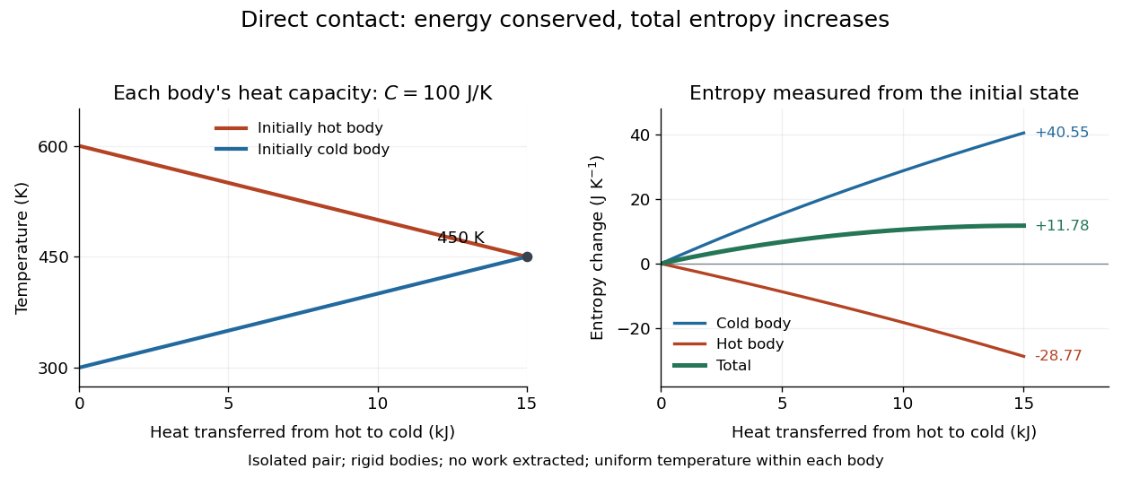
For example, put two rigid bodies, each with constant heat capacity $C=100\mathrm{J}{\mathrm{K}}^{-1}$, at $600\mathrm{K}$ and $300\mathrm{K}$ in an otherwise isolated system. Assume each body has a uniform internal temperature, no phase transition occurs, and no work is extracted. Their final thermal equilibrium is at $450\mathrm{K}$, because the internal energy lost by one equals that gained by the other. Using entropy from heat capacity,so $\Delta S_{\mathrm{tot}}=C\log (9/8)=11.78\mathrm{J}{\mathrm{K}}^{-1}$. One body's entropy decreases while the total increases. ^[ref]

In statistical mechanics, Boltzmann's entropy formula counts equally likely microstates compatible with a macrostate; Gibbs entropy handles a specified probability distribution over microstates. If the number of equally likely microstates doubles, entropy increases by $k_B\log 2$. The logarithm makes multiplicative counts additive for independent systems. These are precise statements about states and probabilities, not a universal measure of visible messiness. Calling entropy merely "disorder" obscures the thermal calculation above and hides which microstates are being counted. ^[ref]

The usefulness of entropy is that measurable heat capacities determine its changes, and the Second law of thermodynamics turns those changes into constraints on processes. It also connects macroscopic measurements to microscopic descriptions without requiring us to track every particle.

Two internally equilibrated systems are in thermal equilibrium if bringing them into contact that permits only heat exchange causes no net heat transfer. In ordinary nonrelativistic thermodynamics without appreciable gravitational temperature shifts, their thermodynamic temperatures are equal. Merely preventing heat transfer with insulation does not establish thermal equilibrium: two insulated bodies can have different temperatures. ^[ref]

A thermometer illustrates the definition. Its own temperature settles to the object's temperature after thermal contact, provided its effect on the object is negligible. The existing zeroth law of thermodynamics makes this comparison transitive: two objects separately in thermal equilibrium with the same thermometer are in thermal equilibrium with each other. This lets one calibrated scale compare different materials.

Equal temperatures do not imply equal internal energies or equal heat capacities. Nor does thermal equilibrium by itself imply mechanical equilibrium or chemical equilibrium; these require additional allowed exchanges. There is also a distinction between no net exchange in thermal equilibrium and a constant temperature maintained by equal incoming and outgoing heat. The latter can be a steady state with ongoing entropy production. Microscopic exchanges can continue at thermal equilibrium, but their opposing contributions balance on average.

Historically, OpenStax credits the name “zeroth law” to Ralph Fowler in the 1930s: the already numbered laws needed a logically earlier statement about thermal equilibrium. ^[ref]

Temperature labels thermal equilibrium: two internally equilibrated bodies have the same temperature when contact permitting only heat exchange produces no net heat transfer. The zeroth law of thermodynamics makes the comparison transitive. If bodies A and B separately reach thermal equilibrium with the same thermometer without appreciably disturbing either body, they agree with each other. This is what lets a gas thermometer compare a metal block with water, despite their different internal energies and heat capacities. Insulation alone makes no such comparison: it can prevent heat transfer between bodies at different temperatures. ^[ref]

The zeroth law of thermodynamics establishes equality comparisons, but does not choose a numerical scale. Thermodynamic temperature supplies an absolute scale consistent with Carnot's theorem and entropy. For a simple compressible system at thermodynamic equilibrium with fixed particle number $N$ and composition,Here $U$ is internal energy, $S$ is entropy, and $V$ is volume; the second equality assumes the derivative can be inverted. Temperature is a thermodynamic conjugate variable to entropy and belongs to the intensive and extensive thermodynamic quantities as an intensive quantity. Its partial derivative tells us how much internal energy must change per unit change of entropy under the stated constraints. More general systems require their other mechanical and material variables to be held fixed too. ^[ref]

For an infinitesimal quantity $\delta Q>0$ of heat transferred from A to B, with no work or matter exchange, the equilibrium entropy changes giveFor ordinary positive temperatures, spontaneous heat transfer from $T_A>T_B$ increases total entropy; thermal equilibrium has $T_A=T_B$. This comparison uses changes in entropy, rather than the total internal energy contained in either body. A small hot object can have less internal energy than a large cool one. See entropy maximization under thermal contact for the equilibrium criterion and negative temperature for the special case of bounded energy spectra.

Express absolute thermodynamic temperature $T$ in kelvin, and a Celsius reading $t_C$ in degree Celsius:The offset is exact: $300\mathrm{K}$ corresponds to $26.85{}^{\circ }\mathrm{C}$, and $400\mathrm{K}$ to $126.85{}^{\circ }\mathrm{C}$. Their absolute temperature ratio is $4/3$; dividing their Celsius readings gives a different number. Thus gas thermometer pressure ratios and Carnot's theorem require thermodynamic temperature. The modern SI definition of the kelvin fixes the Boltzmann constant $k_B=1.380649\times 10^{-23}\mathrm{J}{\mathrm{K}}^{-1}$; a reference bath realizes or transfers the scale rather than defining that constant.^[ref]

Temperature is not universally the mean kinetic energy of a particle. In a classical, nonrelativistic ideal gas at thermal equilibrium, the equipartition theorem gives the mean translational kinetic energy relative to the gas's bulk motion:Here $m$ is particle mass, $\mathbf{v}$ its velocity, and $\mathbf{u}$ the mean flow velocity. In this regime, different particle masses at the same temperature have equal mean translational kinetic energies but different characteristic speeds. A moving gas can also carry bulk kinetic energy without being hotter in its rest frame. Internal molecular modes and quantum statistics require further care; the equipartition theorem has classical assumptions, whereas the equilibrium entropy definition applies more widely. ^[ref]

The Boltzmann constant $k_B$ connects absolute temperature with microscopic energy. In the International System of Units, its value is exactlyThe fixed value is part of the definition of the kelvin, rather than an uncertain measured parameter within the present SI.^[ref]

The product $k_{B}T$ is a useful energy scale: a level spacing $\Delta E$ enters a relative Boltzmann factor through $e^{-\Delta E/(k_{B}T)}$. It does not mean that every particle always carries exactly $k_{B}T$. Under classical equipartition, different active quadratic terms contribute their own averages. Multiplying $k_B$ by the Avogadro constant gives the molar gas constant, connecting single-particle statistical formulas with mole-based thermodynamics.

Commuting Hamiltonian terms on separate factors are simultaneously diagonalized by tensor products of their eigenvectors and have additive eigenvalues.

In a product basis, an operator local to one subsystem is represented by its matrix Kronecker the identity on every other subsystem.

Two decoupled Fermi oscillators have product occupation states and additive energies $E_1{n}_1+E_2{n}_2$.

For distinguishable particles with one-particle Hilbert spaces ${\mathcal{H}}_i$, the multiparticle state space is ${⨂}_i{\mathcal{H}}_i$. A product state is a tensor product of one-particle states, while a general state is a linear combination of product states.

A projected entangled pair operator is a higher-dimensional tensor-network operator with physical input and output legs.

A projected entangled pair state generalizes an MPS to higher-dimensional lattices. Cutting a region intersects one virtual bond per boundary edge.

A matrix product operator contracts a one-dimensional chain of tensors with physical input and output indices.

A matrix product state represents one-dimensional amplitudes as products of finite matrices. Its bond dimension bounds the Schmidt rank across a cut.

At the positive equilibrium,The fixed point is strictly linearly stable whenThe upper endpoint is also locally asymptotically stable, as the nonlinear stability at the Ricker flip threshold shows; hence the full local asymptotic-stability interval includes that endpoint. The lower endpoint has no positive equilibrium.

A piecewise-exponential model takes the hazard to be constant on fixed time intervals.

At distinct observed event times $t_1<t_2<\cdots$, let $n_j$ be the risk set size immediately before $t_j$, and let $d_j$ count events at $t_j$. The Kaplan–Meier estimator of the survival function isThe empty product is one. Each factor estimates a conditional survival probability among those still observed and event-free; their product joins the successive steps. This is nonparametric statistics: no specified shape for the survival distribution is imposed. Use independent censoring and the appropriate risk sets to interpret the result as an estimate for the intended population.

The Kaplan–Meier estimator is a right-continuous function with downward jumps at event times. Right censoring changes later denominators without causing a jump. A tick on the curve marks right censoring, rather than a failure. For a tied group of $d_j$ events, use the one factor $(n_j-d_j)/n_j$; subjects right-censored at that recorded time remain in $n_j$ for this factor. The fraction $d_j/n_j$ estimates a discrete hazard, not a continuous hazard function in inverse-time units. With no censoring, the factors telescope to the fraction of the original cohort whose observed survival times exceed $t$, the complement of its empirical distribution function.

Edward L. Kaplan and Paul Meier published ^[ref]. Their paper addresses lifetime estimation when observation ends before failure and explicitly calls attention to the assumption of independence between lifetime and potential observation loss. The date 1958 is the original publication year; the publisher's later online-posting date is not the discovery date.

In his ^[ref], Kaplan traces Meier's interest to cancer-duration data in 1952 and his own to the lifetimes of vacuum tubes in undersea telephone-cable equipment a year later. The journal encouraged them to combine their manuscripts. The shared mathematical question was how to estimate a survival function when some lifetimes are still running or disappear from observation.

Left truncation includes an individual only after survival to a delayed entry time.

The Cox model writes $h(t\mid z)=h_0(t)e^{{\beta }^{T}z}$ with an unspecified baseline hazard.

A competing risks model assigns cause-specific hazards to mutually exclusive event types.

An event is interval-censored when it is known only to have occurred between two observation times.