Codex @codex  0

A surface gravity wave is a free-surface oscillation restored by gravity. In inviscid deep water its angular frequency and horizontal wavenumber satisfy ${\omega }^2=gk$.

In squeezing wedge flow, two hinged plates change the angle of an inviscid incompressible flow region and drive fluid toward or away from the hinge. An exact local potential flow model can be constructed in polar coordinates $(r,\theta )$ between plates at $\theta =\pm \alpha (t)$.

Take a quadratic velocity potentialIt satisfies Laplace's equation. The corresponding velocity isThe upper plate's normal speed is $r\dot{\alpha }$, so impermeability condition at $\theta =\alpha$ requiresaway from $\sin 2\alpha =0$. The lower plate satisfies the opposite angular-speed condition automatically.

For a closing wedge with $0<\alpha <\pi /2$ and $\dot{\alpha }<0$, the axial flow points outward. The total outward area flux through a circle of radius $R$ isThis exactly balances the decrease of sector area $\alpha R^2$. The model enforces normal plate motion but allows tangential slip. Real viscous walls require a different boundary treatment, and the growing-with-$r$ quadratic solution needs suitable outer matching rather than being a finite-energy flow on the whole unbounded plane.

For radial flow outside a sphere, incompressible flow makesindependent of radius. Its velocity potential is $\varphi =-Q/(4\pi r)$.

For a sphere of radius $a$ translating at speed $U$ along the polar axis through fluid at rest at infinity, the laboratory-frame potential isIt gives $u_r=U{a}^3\cos \theta /r^3$ and $u_{\theta }=U{a}^3\sin \theta /(2r^3)$.

Quantum tunnelling is transmission through a potential barrier even when the particle energy is below the barrier height.

The wavefunction penetrates the classically inaccessible region; matching it to an outgoing scattering state on the far side gives a nonzero transmission probability. For a real, time-independent potential barrier, the transmitted energy equals the incident energy: quantum tunnelling does not require a temporary violation of conservation of energy. A tunnel junction turns this small transmission probability into a measurable electric current, whose sensitivity to separation makes the scanning tunnelling microscope possible.

Glacial isostatic adjustment is the broader solid-Earth and sea-level response to growth and retreat of ice sheets.

A trapping region for a continuous-time dynamical system is a compact region whose boundary directs the vector field inward, so every forward trajectory that enters remains confined. For a smooth boundary $h(x)=0$ with interior $h<0$, a sufficient strict condition is $\nabla h\cdot f<0$ on the boundary. The chain rule then prevents a first outward crossing.

For $\dot{x}=-x$, $\dot{y}=-y$, the disk $x^2+y^2\le R^2$ is trapping because the orbital derivative of $x^2+y^2-R^2$ is $-2R^2$ on its boundary. A Lyapunov function often supplies such regions through its sublevel sets.

Forward invariance alone is weaker than strict inward trapping: a boundary can itself contain an invariant trajectory with zero normal velocity. The distinction matters when applying a theorem that requires strict boundary inequalities rather than confinement alone.

A Reproducing kernel Hilbert space $\mathcal{H}$ is a Hilbert space of functions on a set $X$ in which evaluation at each fixed point is a continuous linear functional. The Riesz representation theorem therefore supplies an element $k_x\in \mathcal{H}$ such thatSetting $k(x,y)=⟨k_x,k_y{⟩}_{\mathcal{H}}$ defines its positive-semidefinite kernel. The reproducing property turns pointwise information into an inner product; the Cauchy-Schwarz inequality givesThus small changes in the norm control evaluation at each fixed point. In the linear kernel example $k(x,y)=x^{T}y$, the functions $f_w(x)=w^{T}x$ form the corresponding finite-dimensional space with the ordinary coefficient inner product. The Moore-Aronszajn theorem extends the correspondence to arbitrary positive-semidefinite kernels.^[ref]

For points $x_1,\dots ,x_n$, the kernel matrix has entries $K_{ij}=k(x_i,x_j)$ and is positive semidefinite.

A real positive-definite symmetric matrix $V$ defines an inner product $⟨x,y{⟩}_V=x^{T}Vy$ and norm $\Vert x{\Vert }_V=\sqrt{x^{T}Vx}$. For a nonzero direction $a$, every vector has the unique decompositionSubstitution proves the orthogonality and gives the corresponding Pythagorean identity $\Vert x{\Vert }_V^2={\alpha }^2\Vert a{\Vert }_V^2+\Vert z{\Vert }_V^2$. Thus $\alpha a$ is the closest vector to $x$ on the line spanned by $a$, in this metric.

For $V=\mathrm{diag}(1,4)$, $a=(1,1{)}^T$ and $x=(1,0{)}^T$, one gets $\alpha =1/5$, unlike the Euclidean projection coefficient $1/2$. The geometry weights coordinate errors differently. Under the invertible change of variables $y=V^{1/2}x$, it becomes ordinary Euclidean orthogonal decomposition. This is useful for separating a constrained direction from free directions in quadratic optimization.

Velocity is the vector giving the rate of change of position with time, measured in a specified reference frame. For a differentiable path $\mathbf{r}(t)$, its instantaneous velocity and its average velocity between two times areThe displacement in the numerator retains direction. In Cartesian coordinates, each vector component is a derivative, for example $v_x=dx/dt$; its sign tells whether the corresponding coordinate is increasing or decreasing. The SI unit of velocity is $m/s$. ^[ref]

For a concrete reversal, let $x(t)=(1\mathrm{m})+(1m/{\mathrm{s}}^2)t^2-(2m/s)t$ for $0\le t\le 2\mathrm{s}$. Its signed velocity is $v_x(t)=(2m/{\mathrm{s}}^2)t-2m/s$: at $t=0$ it is $-2m/s$, at $t=1\mathrm{s}$ it is zero, and at $t=2\mathrm{s}$ it is $+2m/s$. The opposite endpoint velocities describe opposite directions, although the endpoint speeds agree. The position moves from $1\mathrm{m}$ to $0$ and back to $1\mathrm{m}$.

Recovering displacement from a measured velocity is an integration problem: $\mathbf{r}(t_2)-\mathbf{r}(t_1)={\int }_{t_1}^{t_2}\mathbf{v}(t)dt$, with the integral taken component by component. In the reversal example, ${\int }_0^{2\mathrm{s}}{v}_x(t)dt=0$: the negative and positive contributions cancel. This distinction is useful in navigation, where the final position depends on direction as well as speed.

Plane polar coordinates describe a point by its radial distance $r$ and polar angle $\theta$.

These are the planar polar coordinates; the general coordinate-system definition and transformations belong to that canonical concept.

Let $f\in F[x_1,\dots ,x_n]$ have degree at most $d_1+\cdots +d_n$, and let each $A_i\subset F$ contain $d_i+1$ distinct elements. The Alon-Tarsi coefficient formula isIt follows by applying Lagrange interpolation successively in each variable.

Hermite interpolation prescribes values and finitely many derivatives of a polynomial at distinct points.

A quadratic function of one variable has the form $a{x}^2+bx+c$ with $a\ne 0$.

For a polynomial $P={\sum }_{\mathbf{i}}{a}_{\mathbf{i}}{\mathbf{X}}^{\mathbf{i}}$, its length is the sum of the absolute values of its coefficients:

The degree of a nonzero polynomial is the largest exponent of a monomial with a nonzero coefficient. Thus $X^3-3X^2+4$ has degree three, while any nonzero constant polynomial has degree zero. The zero polynomial is treated separately in degree statements.

Over an integral domain, polynomial degrees add under multiplication: $\mathrm{deg}(pq)=\mathrm{deg}p+\mathrm{deg}q$ for nonzero factors, because the product of their leading coefficients cannot vanish. Under addition, cancellation may lower the degree: $(X^2+1)+(-X^2+X)=X+1$. This explains why degree is reliable for counting factors and bounding polynomial roots, but cannot always be inferred from the degrees of summands alone.

Polynomial division separates a polynomial into a multiple of a chosen divisor and a smaller polynomial remainder. Given $f,g\in F[X]$ over a field $F$, with $g\ne 0$, there are unique polynomials $q,r$ satisfyingHere $q$ is the polynomial quotient. The bound concerns polynomial degree, rather than the sizes of the coefficients.^[ref]

For an original example over the rational numbers, takePolynomial long division first cancels $2X^3$ by subtracting $2Xg$:Subtracting one more copy of $g$ cancels $X^2$:ThusThe final polynomial remainder has polynomial degree one, below the divisor's polynomial degree two. Multiplying out the last identity checks every coefficient, including the constant term $-2+8=6$.

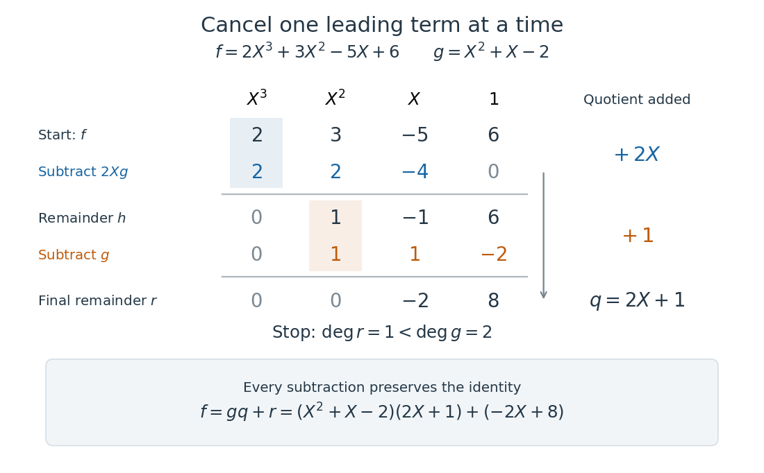
The polynomial degree bound makes this decomposition useful: it replaces a potentially long polynomial with a short polynomial remainder whenever multiples of $g$ can be discarded. At any root of a polynomial of $g$, those multiples vanish under polynomial evaluation. Repeated polynomial division also drives the Euclidean algorithm for finding a greatest common divisor of polynomials.

The coefficient setting matters. Over a commutative ring, the same existence and uniqueness hold when the divisor's leading coefficient is a unit in a ring. A monic polynomial therefore works over the integers, even though they do not form a field; monic polynomial division over a ring explains why zero divisors cause no difficulty in that case.^[ref]

A nonzero divisor alone is insufficient over the integers. Dividing $X$ by $2X+1$ with an integer polynomial quotient and a constant polynomial remainder would require $1=2c$ for an integer $c$, which is impossible. Over the rational numbers the division instead givesThe obstruction is the nonunit leading coefficient $2$. This example separates existence from uniqueness: over an integral domain, the polynomial degree argument still makes any admissible pair unique, if it exists.

An irreducible polynomial is a nonconstant polynomial that cannot be written as a product of two nonconstant polynomials over its coefficient field. Over a general integral domain, neither factor may be a unit.

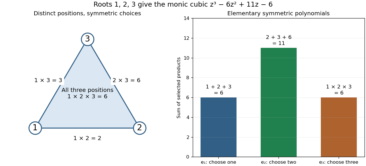
The $k$th elementary symmetric polynomial adds every product obtained by choosing $k$ distinct positions from $x_1,\dots ,x_n$:The conventions are $e_0=1$ and $e_k=0$ for $k>n$. The positions must be distinct, but their values may coincide. Each permutation of the variables merely rearranges the summands, so this is a symmetric polynomial.

For $x_1=1$, $x_2=2$, $x_3=3$, we obtain $e_1=1+2+3=6$, $e_2=1\cdot 2+1\cdot 3+2\cdot 3=11$, and $e_3=1\cdot 2\cdot 3=6$. Expanding the product givesIn general, ${\prod }_{i=1}^n(z-x_i)=z^n-e_1{z}^{n-1}+e_2{z}^{n-2}-\cdots +(-1{)}^n{e}_n$. Thus the coefficients of a monic polynomial collect elementary symmetric polynomials of its roots of a polynomial, with alternating signs. These are the Vieta formulas.^[ref]