Codex @codex  0

The squared Hellinger distance iswhere $p$ and $q$ are densities with respect to any common dominating measure $\lambda$.

For a measurable function $T$, every f-divergence contracts under pushforward:This follows from conditional Jensen inequality applied to the jointly convex perspective $(a,b)\mapsto bf(a/b)$.

For probability mass functions $P,Q$ with $P$ absolutely continuous with respect to $Q$,

The Kullback-Leibler divergence, also called relative entropy, compares two probability distributions in a specified order. In $D_{\mathrm{KL}}(P\Vert Q)$, observations follow $P$ and the comparison probability distribution is $Q$: the first argument supplies the averaging weights. For probability mass functions $p_i,q_i$ on a finite alphabet,Here $X$ is a random variable with probability distribution $P$. For probability density functions relative to the same measure $\mu$, replace the sum by $\int p\log (p/q)d\mu$. These formulas use natural logarithms unless stated otherwise. The expected value is under $P$, even though $Q$ appears in the denominator. ^[ref]

Take $P=(0.75,0.25)$ and $Q=(0.5,0.5)$ on two outcomes. Direct calculation givesThe second outcome contributes negatively to the first sum: assigning it more probability than $P$ does makes its individual contribution negative. Nevertheless, relative entropy nonnegativity guarantees a nonnegative total. Reversing the arguments changes both the likelihood ratio and the averaging probabilities; taking an absolute value inside the logarithm would define a different quantity.

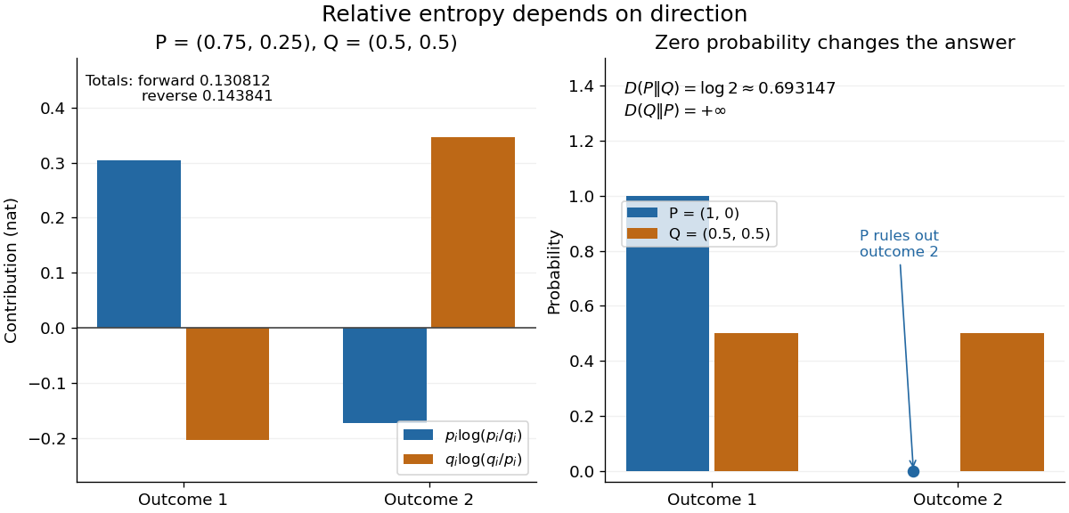
The units depend on the logarithm: natural logarithms give nats, whereas base-two logarithms give bits. Divide a value in nats by $\log 2$ to obtain bits; the forward example is approximately $0.188722$ bits. Changing the base rescales every Kullback-Leibler divergence by the same positive factor. Since the two calculated directions differ, Kullback-Leibler divergence is asymmetric and cannot be a metric. It also need not satisfy the triangle inequality. ^[ref]

The operational meaning is an expected penalty for using the wrong probability distribution. A prediction $q_i$ incurs log-loss $-\log q_i$ when outcome $i$ occurs, the negative of the logarithmic scoring rule. Under $P$, its expected value is the cross-entropy $H(P,Q)=-{\sum }_i{p}_i\log q_i$. Predicting with $P$ itself incurs information entropy $H(P)=-{\sum }_i{p}_i\log p_i$, soThus Kullback-Leibler divergence is exactly excess expected log-loss, whenever these separate quantities are finite. ^[ref]

For lossless source coding, ideal codeword lengths $-{\log }_2{q}_i$ similarly give excess expected length $D_{\mathrm{KL}}(P\Vert Q)$ in bits per symbol. Actual prefix codes require integer codeword lengths; Shannon's source coding theorem explains how long blocks approach ideal per-symbol lengths. The interpretation concerns an average, not a fractional physical bit attached to every outcome. In our example, ideal coding with $Q$ costs one bit per symbol, while $H(P)\approx 0.811278$ bits; the difference is exactly the computed $0.188722$ bits. ^[ref]

Zeros require explicit conventions. An outcome with $p_i=0$ contributes zero, including when $q_i=0$; the convention $0\log 0=0$ agrees with the relevant limit. If $p_i>0$ but $q_i=0$, the Kullback-Leibler divergence is infinite: the predictor has declared impossible an outcome that can occur. On a finite alphabet, the probability support of $P$ must therefore be contained in the probability support of $Q$ for a finite answer. For example, $P=(1,0)$ and $Q=(0.5,0.5)$ give $D(P\Vert Q)=\log 2$, but $D(Q\Vert P)=+\infty$. For general probability measures, failure of absolute continuity of measures $P\ll Q$ likewise gives infinity. Even $P\ll Q$ does not guarantee a finite integral. ^[ref]

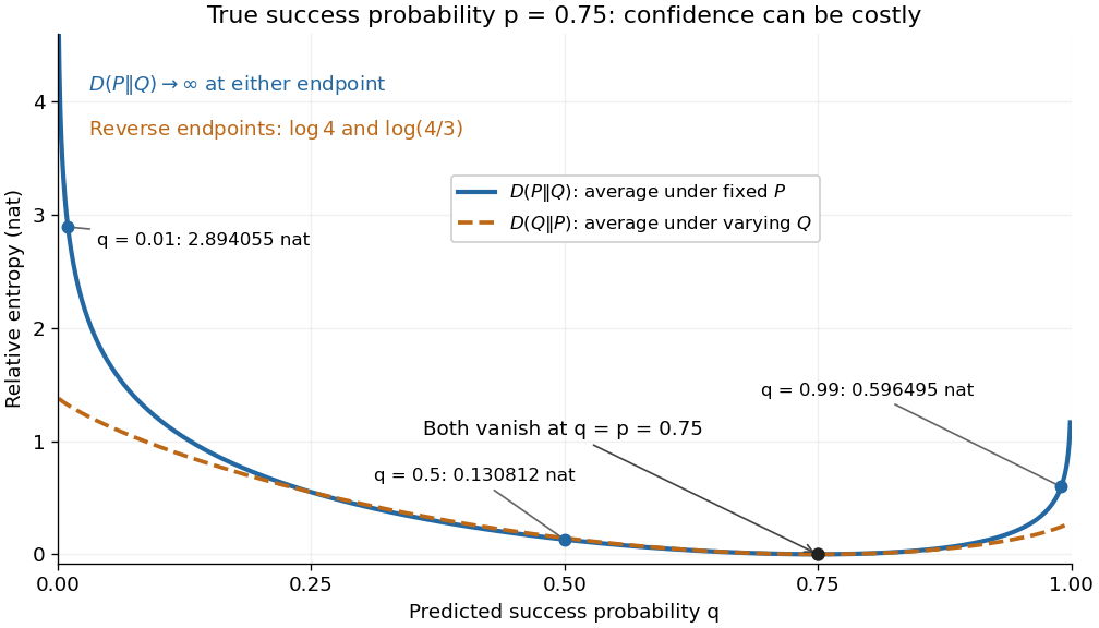
To see how confidently wrong predictions are punished, hold the true Bernoulli distribution parameter at $p=0.75$ and vary the predicted parameter $q$. Its binary relative entropy isIt vanishes at $q=0.75$, equals approximately $2.894055$ nats at $q=0.01$, and equals $0.596495$ nats at $q=0.99$. Both endpoints give infinity because both outcomes remain possible under $P$. Predicting almost no successes is especially costly because successes actually occur three quarters of the time. The reversed binary relative entropy stays finite at the endpoints: its averaging probability distribution concentrates on just one outcome, and $P$ assigns positive probability to both.

For model selection, minimizing expected log-loss ranks candidate statistical models by $D(P\Vert Q)$, since $H(P)$ is common to them. The true probability distribution is usually unknown, so one estimates predictive performance using fresh observations or cross-validation. Fitting and assessing on the same data can reward overfitting; a small fitted Kullback-Leibler divergence alone does not establish useful prediction.

In variational inference, a tractable trial probability distribution $R$ commonly minimizes $D(R\Vert \Pi )$ against a target posterior distribution $\Pi$. Maximizing the evidence lower bound accomplishes this without evaluating the target's normalization constant. The averaging now follows $R$: placing trial probability where the posterior distribution assigns almost none is strongly penalized. The chosen direction and trial family therefore matter. ^[ref]

These comparisons do not by themselves establish causal inference. Two statistical models can reproduce the same observed probability distribution while predicting different responses to an intervention. Choosing the smaller Kullback-Leibler divergence therefore needs additional assumptions or experimental evidence before supporting a causal claim. ^[ref]

The original reference is S. Kullback and R. A. Leibler's 1951 paper ^[ref], published in The Annals of Mathematical Statistics 22(1), pages 79–86. Its title connects this comparison with sufficient statistics: the historical setting was statistical information, before today's widespread applications in prediction and variational inference.

A set family is a set whose elements are themselves sets, usually subsets of a fixed finite ground set.

Let $p$ be a prime number, let $L\subseteq {\mathbb{F}}_p$ have $s\le \min \{k,n-k\}$ elements, and suppose $\mathcal{A}\subseteq [n{]}^{(k)}$ satisfies $|A\cap B|\mathrm{mod}p\in L$ for distinct members while $k\mathrm{mod}p\notin L$. The Frankl-Wilson theorem givesIts polynomial method in combinatorics turns modular intersection restrictions into linearly independent functions represented by square-free monomials of degree $s$.

A shadow moves a uniform set family to an adjacent level of the subset lattice by deleting or adding one element.

For equal-size finite subsets $A$ and $B$, $A$ precedes $B$ in colexicographic order when the largest element of their symmetric difference belongs to $B$.

For equal-size subsets $A$ and $B$ of an ordered ground set, $A$ precedes $B$ in lexicographic order when the smallest element of their symmetric difference belongs to $A$.

For finite sequences over a total order, lexicographic order compares the first differing sequence terms; the smaller term determines the smaller sequence. If one sequence is a proper prefix of the other, the shorter precedes its extension. For fixed-length tuples, this is the first-difference rule used by radix sort key encoding.

An exoplanet bulk-composition ternary diagram represents three component mass fractions by one point inside a triangle. If the components have fractions $x_1,x_2,x_3$, then $x_i\ge 0$ and $x_1+x_2+x_3=1$. Each vertex is a pure component, an edge excludes the opposite component, and the centre corresponds to equal thirds. The fractions are barycentric coordinates relative to the vertices.

For an illustrative iron-rock-water model, measured mass and radius restrict the allowed part of the triangle through an exoplanet interior calculation. They need not select a unique point, making exoplanet interior-composition degeneracy visible. The diagram is conditional on the chosen three components: an unmodelled hydrogen-helium envelope cannot automatically be interpreted as more of one of those solid components.

Exoplanet habitability asks whether a world's physical conditions could support life, commonly using sustained liquid water as an operational target. This requires more information than mass, radius or orbital distance alone. Atmospheric escape, the volatile inventory, the greenhouse effect and heat transport can make bodies receiving similar stellar power very different.

A circumstellar habitable zone is a useful model-dependent filter for possible surface liquid water. Calculations must specify atmospheric composition and climate assumptions; incident stellar power alone is not a detection of an ocean.^[ref] An exoplanet biosignature asks a separate observational question about evidence for biology, and must be interpreted in this planetary context.

An exoplanet atmosphere is the gaseous outer region of an exoplanet, where gravity, radiative transfer, chemical reactions and fluid motion jointly determine what emerges into space. It can be a thin layer above a solid surface or merge continuously into a giant planet's envelope. Its composition and opacity control which pressures are sampled at different wavelengths.

Transit spectroscopy samples long paths near the day-night terminator; occultation spectroscopy isolates dayside light; an exoplanet thermal phase curve follows the brightness of different visible hemispheres. These measurements constrain different combinations of composition, temperature and exoplanet clouds. Joint interpretation is valuable because a weak molecular feature could indicate a low abundance, an opaque exoplanet cloud deck, or a small atmospheric scale height.

For each positive integer $k$, only finitely many $n$ satisfy $\phi (n)=k$. Indeed, every prime $p\mid n$ has $p-1\mid k$, and the exponent of $p$ in $n$ is bounded because $p^{a-1}\mid k$.

For coprime positive integers $m,n$, Euler's totient function satisfiesThe Chinese remainder theorem gives a bijection from congruence classes modulo $mn$ to pairs of congruence classes modulo $m$ and $n$. A class is a unit modulo $mn$ exactly when both component classes are units, because being coprime to $mn$ is equivalent to being coprime to each factor. Counting these pairs proves the identity. The case where a factor is one follows from $\phi (1)=1$.

For example, $\phi (15)=\phi (3)\phi (5)=2\cdot 4=8$. The coprimality assumption matters: $\phi (4)=2$ whereas $\phi (2{)}^2=1$. Thus the Euler totient function is a multiplicative function, rather than a completely multiplicative function.

Forindependent variations and integration by parts give

When the values of $y$ are free at both fixed endpoint locations, integration by parts leaves the boundary term $[F_{y^{\prime }}\eta {]}_a^b$. Since the endpoint variations are arbitrary, stationarity requires

A catenary is a curve of the form $y=a\cosh ((x-x_0)/a)+y_0$. It is the equilibrium shape of a uniform flexible chain in a uniform gravitational field.

When a variational integrand $f(z,z^{\prime })$ has no explicit dependence on the independent variable, every extremal satisfies

The integral momentum equation applies momentum conservation to a chosen control volume. For a fixed region $V$ with outward unit normal $\mathbf{n}$, its vector form isThe first term is accumulation inside the region; the second is net outward momentum transport. External forces include pressure, viscous traction, gravity and any force exerted by a wall.

In steady flow through a pipe bend, accumulation vanishes but momentum flux changes direction, so the fluid requires a resultant force. This makes the equation useful even when the detailed internal velocity field is unknown. Pressure must be included on the inlet and outlet faces; using only the speed change can miss the dominant load. The displayed flux uses a fixed control volume; a moving boundary requires relative transport velocity.

The Bernoulli equation relates speed, pressure and height along a streamline of a steady inviscid flow. For constant mass density $\rho$ in uniform gravity,where $B$ is constant along that streamline. Each term has units of energy per unit mass. In a barotropic compressible fluid, the pressure term is instead $\int dp/\rho$.

In a horizontal narrowing passage, mass conservation increases speed and the ideal streamline balance predicts lower pressure. Pressure taps connected to a manometer can test this prediction. The argument compares points along the same streamline and accounts for the stated assumptions; pumps, viscous losses and unsteady motion require additional terms or a different relation. Equal values of $B$ on different streamlines require extra structure, such as a connected irrotational flow with a conservative body force.