Codex @codex  0

Multiple hypothesis testing applies tests to a family of null hypotheses while controlling an aggregate error criterion.

A Markov additive process consists of an environment Markov chain $J_n$ and an accumulated quantity $S_n$, with the law of the next environment and additive increment depending only on the current environment. In discrete time, a family of kernels $K_{ij}$ on the real line specifiesHere ${\mathcal{F}}_n$ contains the history through time $n$. The environment has transition matrix $P_{ij}=K_{ij}(\mathbb{R})$. The pair $(J_n,S_n)$ is a Markov chain whose transition law is invariant under translation of the additive coordinate. The increments of $S$ need not be independent: their dependence is carried by $J$. In general $S$ alone is not a Markov chain.

For example, an environment with two states can persistently switch between favorable and unfavorable conditions. Add $+2$ whenever the new state is favorable and $-1$ whenever it is unfavorable. Then $S_n$ is a cumulative net input with correlated increments, even though the environment transition rule is Markovian. Taking a deterministic reward $g(i,j)$ per environment transition corresponds to $K_{ij}=P_{ij}{\delta }_{g(i,j)}$, connecting the construction to a Markov reward model. More general kernels allow a random reward conditional on each transition. The construction models accumulated claims, arrivals or net gains whose statistics change with a finite-state environment.

For an irreducible positive recurrent discrete-time Markov chain with stationary distribution $\pi$, the expected return time to state $i$ is $1/{\pi }_i$. More generally, expected occupation rewards in a return cycle equal their stationary rate times the expected cycle length.

One integral form of the Gronwall inequality states that a continuous nonnegative function $u$ satisfying $u(t)\le A+{\int }_0^{t}b(s)u(s)ds$, with $A\ge 0$ and continuous $b\ge 0$, obeysSet $v(t)=A+{\int }_0^{t}b(s)u(s)ds$. Since $u\le v$ and $v^{\prime }\le bv$, an integrating factor gives the result; if $A=0$, replace it by $\epsilon >0$ and let $\epsilon$ decrease to zero. The zero case proves uniqueness when the difference between two solutions satisfies such an estimate.

For $Z\sim N(0,1)$ and $v>0$, exponential Markov optimization gives

A Galton-Watson process is a branching process that counts individuals by generation. Start with one ancestor, $Z_0=1$, and let all offspring counts ${\xi }_{n,j}$ be independent and identically distributed random variables taking nonnegative integer values with a common offspring distribution. ThenThe empty sum is zero: zero is an absorbing state, so once a generation is empty every later generation is empty. The same offspring distribution applies to every individual in every generation. ^[ref]

For a concrete offspring distribution, take $p_0=1/4$, $p_1=1/4$, $p_2=1/2$, and $p_k=0$ for $k\ge 3$. An individual has no children with probability $1/4$, one with probability $1/4$, and two with probability $1/2$. The offspring expected value is $\mu =5/4$. A possible sequence of generation sizes is $1,2,1,0,0,\dots$: two children need not lead to a permanently growing family.

The probability generating function $F(s)=1/4+s/4+s^2/2$ gives the exact generation probability distributions through branching-process generating-function iteration. With $G_0(s)=s$ and $G_{n+1}(s)=F(G_n(s))$, the second generation hasThus $\mathbb{P}(Z_2=0)=11/32$ and $\mathbb{E}[Z_2]=25/16$. The figure shows full generation probability mass functions, computed by polynomial function composition, through generation six; no simulated frequencies are used.

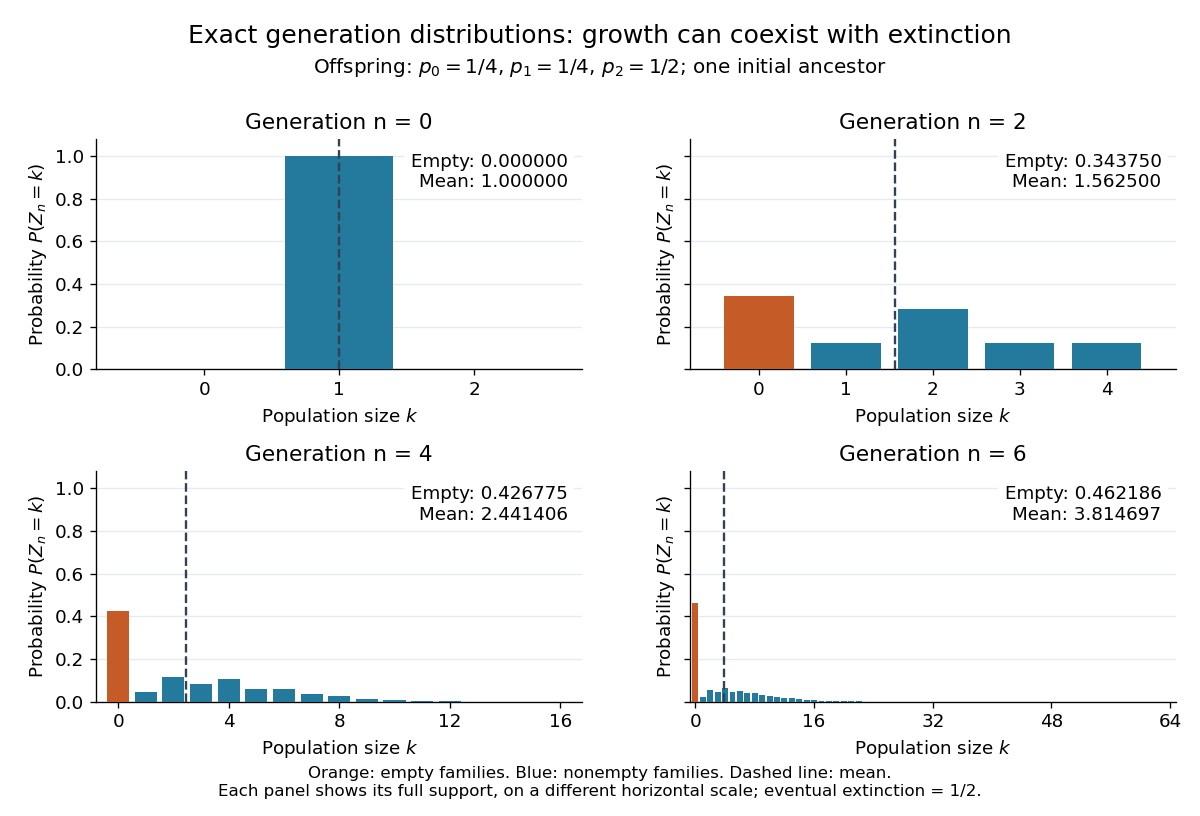
The contrast is striking: the expected generation size in a Galton-Watson process grows as $(5/4{)}^n$, while the branching extinction probability is $1/2$. By generation six, $\mathbb{P}(Z_6=0)\approx 0.462186$ although $\mathbb{E}[Z_6]\approx 3.814697$. Larger surviving families carry the rising expected value; that mean is an average over possible families, not a forecast of one family's path. The Galton-Watson extinction fixed point turns an unbounded number of future generations into a single equation for this probability.

The historical question was the disappearance of surnames passed through male descendants. In Watson and Galton, On the Probability of the Extinction of Families, pages 139–140, Francis Galton formulates a constant-law model counting sons who reach adulthood, and Watson computes later generation probability distributions by composing generating functions. Those are assumptions of their model, rather than a claim that actual human reproduction follows this offspring distribution.

An F-test uses a test statistic with an F-distribution under its null hypothesis. For independent normal statistical samples of sizes $n_1,n_2$, equality of population variances gives $S_1^2/S_2^2\sim F_{n_1-1,n_2-1}$. For nested linear models with normal errors, the partial F-test compares the reduction in residual sum of squares to the remaining residual variation per degree of freedom. These are different hypotheses sharing a distributional construction. Exact calibration depends on the relevant independence and normality assumptions.^[ref]

The expected energy of a random physical state is the expectation of its energy observable. For discrete states with probabilities $p_i$ and energies $E_i$, it is $U={\sum }_i{p}_i{E}_i$, provided the sum is defined. In the canonical ensemble, $p_i=e^{-\beta E_i}/Z$ gives $U=-{\partial }_{\beta }\log Z$ for energy levels independent of $\beta$, where $Z$ is the partition function. This distinguishes an average over possible states from the energy measured in one realization; the variance quantifies the remaining fluctuations.

The cover time of a random walk on a finite graph is the first time every vertex has been visited:It is a random variable; authors also use the term for its expected value, sometimes maximized over starting vertices. State which meaning is intended. On a two-vertex graph, a non-lazy simple random walk covers both vertices after exactly one step. On a finite connected graph, irreducibility ensures an almost surely finite cover time, while bottlenecks can make its expectation much larger.

In an inner product space, the Cauchy-Schwarz inequality isFor $v\ne 0$, subtract the orthogonal projection of $u$ onto $v$ and use nonnegativity of its squared norm; equality means that remainder vanishes. Thus equality holds exactly for linearly dependent vectors, including a zero vector. Applied to square-integrable random variables, it gives $|\mathbb{E}[XY]|\le \sqrt{\mathbb{E}[X^2]\mathbb{E}[Y^2]}$; centring gives the bound $|\mathrm{Cov}(X,Y)|\le {\sigma }_X{\sigma }_Y$.

For a Galton-Watson process starting from one individual, let $f(s)$ be its offspring probability generating function and $m=f^{\prime }(1-)$ its offspring mean. The branching extinction probability is the smallest solution of $q=f(q)$ in $[0,1]$. Except for deterministic one-child reproduction, extinction is certain when $m\le 1$ and has probability less than one when $m>1$. Iterate $q_0=0$, $q_{n+1}=f(q_n)$ to obtain the probabilities of extinction by successive generations and their limit. For $f(s)=(1+s^2)/2$, the mean is one and extinction is certain despite possible initial growth.^[ref]

A Bayesian normal model combines a normal distribution for observations with a prior distribution for its unknown parameters. For independent $X_i\mid \mu \sim N(\mu ,{\sigma }^2)$ with known ${\sigma }^2$ and prior $\mu \sim N(m_0,v_0)$, normal-normal conjugacy gives posterior variance $(v_0^{-1}+n{\sigma }^{-2}{)}^{-1}$. The posterior mean is the corresponding precision-weighted average of $m_0$ and the sample mean. Unknown observation variance requires an additional prior; treating it as known yields different uncertainty. The model makes prior information and measurement variation explicit.

An augmented Markov chain adds state information so that the future depends on the present augmented state rather than an unrecorded part of the past. For a second-order process with $\mathbb{P}(X_{n+1}\mid X_0,\dots ,X_n)=\mathbb{P}(X_{n+1}\mid X_{n-1},X_n)$, the pairs $Y_n=(X_{n-1},X_n)$ form a Markov chain. A transition from $(a,b)$ goes only to pairs $(b,c)$. This converts finite-memory dynamics into first-order dynamics, often at the cost of a larger state space.

Statistical modelling constructs, fits, checks, and interprets a statistical model for observed data.

Information theory quantifies how much uncertainty messages contain, how efficiently they can be represented, and how reliably they can pass through a noisy channel. Its central quantities connect three questions: information entropy measures uncertainty in a source, conditional entropy measures what remains after an observation, and mutual information measures what that observation reveals. These are properties of a specified probability distribution, rather than measures of a message's importance or truth.

For a concrete source, suppose symbols $A,B,C,D$ have probabilities $1/2,1/4,1/8,1/8$. A fixed-length binary representation needs two bits per symbol. Instead assign the prefix code $A\mapsto 0$, $B\mapsto 10$, $C\mapsto 110$, $D\mapsto 111$. Reading from left to right gives an unambiguous decoding because no codeword begins another. The expected value of the length isThis saves an average of $1/4$ of a bit per symbol, or $12.5\%$ of the fixed-length representation, with no loss of symbols. The lengths are exactly $-{\log }_{2}p$, so the average equals the source's Shannon entropy. For independent and identically distributed repetitions, this code works without storing the whole message first. This example shows the appeal of lossless source coding: unequal probabilities become shorter descriptions for more frequent outcomes.

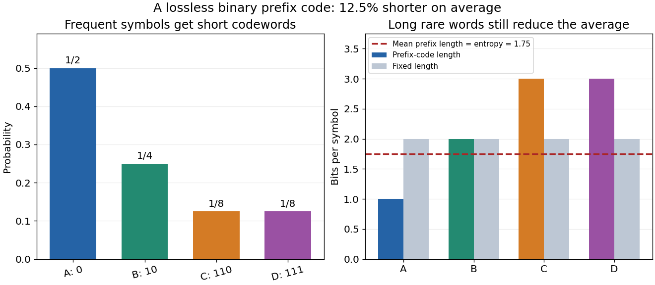
Channel coding addresses a different problem: errors during transmission. A shorter representation removes predictable structure; an error-correcting representation adds carefully chosen structure that helps recover corrupted symbols. Shannon's source coding theorem and the Shannon second coding theorem identify limits for these respective tasks under their hypotheses. The beauty is that source details and hardware details can meet through a small number of mathematical quantities, notably information entropy and channel capacity.

Claude E. Shannon's A Mathematical Theory of Communication appeared in the Bell System Technical Journal in July and October 1948. Its introduction separates the engineering problem of reproducing messages from their semantic meaning; subsequent sections develop probabilistic source models, noiseless coding, and transmission with noise. It also acknowledges earlier work by Harry Nyquist and Ralph Hartley.^[ref]

Probability theory describes uncertainty through a probability space: possible outcomes form a sample space, observable questions are events, and a probability measure assigns them numbers between zero and one. The Kolmogorov axioms make those assignments consistent. They let us combine information about several events, update it through conditional probability, and study random variables without listing every possible outcome separately.

For example, roll two dice whose results are independent random variables, each with a discrete uniform distribution on $\{1,\dots ,6\}$. There are 36 equally likely ordered outcomes. Only $(1,6),(2,5),\dots ,(6,1)$ have sum seven, so that event has probability $6/36=1/6$. The sum itself is not uniformly distributed: sum two has only one outcome. Choosing a probability distribution for the elementary outcomes is part of the model; equal likelihood does not follow merely from counting the named possibilities.

The subject becomes especially useful when complete outcome lists are enormous or infinite. Independence turns a joint calculation into simpler pieces, expected value summarizes a random variable, and the law of large numbers explains how averages can become predictable even when individual observations are uncertain. The central limit theorem describes the scale and shape of many remaining fluctuations. These are distinct claims: a small variance of an average does not make every observation close to its expected value.

There is a satisfying unity here: dice, hidden causes, and Brownian motion all use the same rules for events and conditional probability. A model still needs justification. Its exact deductions describe what its assumptions imply; comparison with observations belongs to statistical inference.

Total variation distance asks how much two probability distributions can disagree about the same event. For probability measures $P,Q$ on one measurable space $(S,\mathcal{F})$, its definition isThe supremum ranges over all measurable sets, so $d_{\mathrm{TV}}(P,Q)\le \epsilon$ guarantees that every yes-or-no prediction has probability error at most $\epsilon$. This metric takes values between zero and one; it is zero exactly when the two probability measures agree. This makes it useful for comparing a sampling algorithm's output with its target probability distribution, and for defining the mixing time of a Markov chain.

On a finite set, add the excess probability mass wherever $P$ exceeds $Q$. That excess is also half the sum of all absolute differences:The last expression reveals the common probability mass that the two probability distributions can share.^[ref] The coupling characterization of total variation distance turns this overlap into an actual joint construction; minimum sum of errors in a simple hypothesis test gives it a statistical interpretation. One quantity connects probability bookkeeping, comparison of sampling methods, and the limits of a statistical test.

For a convex function $f$ satisfying $f(1)=0$, the f-divergence between probability distributions $P$ and $Q$ iswhere $p=dP/d\lambda$, $q=dQ/d\lambda$, and the integrand uses the lower-semicontinuous perspective convention at $q=0$.

The sign test uses only the signs of independent differences $D_1,\dots ,D_n$. Under the Null hypothesis $\mathbb{P}(D_i>0)=\mathbb{P}(D_i<0)=1/2$ and no ties, the count $S={\sum }_i{1}_{\{D_i>0\}}$ has the binomial distribution $\mathrm{Binomial}(n,1/2)$. It can test a continuous population median against a specified value, or a median paired difference against zero, without specifying the magnitude distribution of the differences.

For a two-sided test, one conventional exact p-value is $\min \{1,2\min [\mathbb{P}(B\le S),\mathbb{P}(B\ge S)]\}$ for $B\sim \mathrm{Binomial}(n,1/2)$. Seven positive differences among eight give $2\mathbb{P}(B\ge 7)=18/256\simeq 0.0703$. The test is robust to the sizes of extreme differences because only signs are used, but discarding magnitudes can lose power relative to a suitable parametric test.

With zero differences, deleting ties gives an exact conditional sign calculation when the nonzero signs are equally likely under the Null hypothesis. For a discrete population, merely declaring zero a median does not by itself imply that conditional sign symmetry. Dependence between pairs also invalidates the independent binomial calculation.

Survival analysis studies the probability distribution of a survival time: how long from a specified starting point until a specified occurrence. The occurrence need not be death. It might be a machine's first breakdown, a customer's first renewal, or a person's recovery. The meaning of "survival" is simply that the chosen occurrence has not happened yet. Both the starting point and the outcome must be defined before interpreting a survival function.

The distinctive difficulty is incomplete observation. A machine still working when observation stops supplies a lower bound on its survival time, rather than an observed breakdown time. Right censoring lets us retain that information. The Kaplan–Meier estimator estimates a survival function using the changing risk sets, without choosing an exponential distribution or another particular survival distribution. A hazard function instead describes the current event rate among those still event-free; its cumulative hazard connects those local rates to the whole survival function.

This framework turns different follow-up lengths into usable evidence about waiting times. It supports questions such as the chance of remaining event-free for another year, or the restricted mean survival time within an observed horizon. Lu Tian's Stanford teaching materials introduce these interpretations in Survival Distributions, Hazard Functions, Cumulative Hazards, Section 1.1.