A rectangular potential barrier is the piecewise-constant special case used for exact transmission and reflection calculations.
A piecewise constant barrier of finite width. Exact scattering follows by matching the wavefunction and its derivative at its two interfaces; below its height the internal wave number is imaginary.
Quantum tunnelling is transmission through a potential barrier even when the particle energy is below the barrier height.
The wavefunction penetrates the classically inaccessible region; matching it to an outgoing scattering state on the far side gives a nonzero transmission probability. For a real, time-independent potential barrier, the transmitted energy equals the incident energy: quantum tunnelling does not require a temporary violation of conservation of energy. A tunnel junction turns this small transmission probability into a measurable electric current, whose sensitivity to separation makes the scanning tunnelling microscope possible.
Finite lifetime of an island state due to tunnelling into leads gives an energy-width scale of order . The numerical factor depends on whether denotes a population decay rate, an amplitude decay rate or a sum of partial rates.
Transport by successive real charge-state changes across weak tunnel barriers. Charge electrochemical potentials must enter the source-drain bias window; outside it sequential transport is Coulomb blocked. Higher-order virtual cotunnelling is a distinct process.
At energy equal to a finite rectangular barrier height, the stationary interior Schrödinger equation has a linear solution . Its probability current can be nonzero: . Setting the interior classical kinetic energy to zero does not set the transmitted quantum flux to zero.
A biased double-barrier structure whose intermediate quasi-bound levels control transmission from reservoirs. Bias-dependent alignment can produce negative differential resistance when a resonance moves out of the available injection window.
Suppression of tunnelling because adding or removing a discrete island charge costs more energy than the accessible transport and thermal energy window. Weak junction coupling and small island capacitance make it observable.
A higher-order tunnelling process through intermediate virtual charge states. It can produce transport inside a region where sequential first-order tunnelling is suppressed by Coulomb blockade. Its relevance grows as junction coupling increases.
The electrostatic scale for placing one elementary charge on a capacitance , conventionally . The discrete second difference of the quadratic island energy is , which is the charging contribution to successive-electron addition energies. State the convention when comparing numerical values.
A model with charge-independent total capacitance and a separate single-particle orbital spectrum. An addition energy is , whereas the conventional electrostatic charging scale is . The factor of two should not be confused with diamond full height.
With , the addition electrochemical potential is . Gate and lead voltages enter . Adjacent addition potentials differ by an orbital spacing plus .
A blocked region in a source-drain-voltage versus gate-voltage diagram of a small charge island. Gate widths, edge slopes and tip heights encode gate coupling, junction capacitance ratios and addition energies; extracting named source/drain values requires a bias convention.
With source biased and drain grounded, a constant-interaction island has diamond edge slopes and . The latter includes the gate capacitance. A gate period for charging without an orbital gap is . Combining widths and slopes determines capacitances only under a stated bias and single-island model; shell gaps must not be mistaken for a universal gate period.
Field electron emission releases electrons from matter through electric-field-assisted quantum tunnelling at the surface. The emission mechanism and its rate are distinct from the subsequent acceleration and Larmor formula radiation of an electron already travelling through an approximately uniform electric field.
Quantum tunnelling between different energy bands, including transfer between the valence band and conduction band in a tunnel diode.
Take a nonrelativistic particle of constant mass with energy , and choose the same zero of potential energy on both sides of a rectangular potential barrier:The equality of the exterior potential energies matters: it gives the same exterior wavenumber and makes . Here is the reduced Planck constant. This model has a finite jump in potential energy, no delta potential, and no absorbing term.
For , the time-independent Schrödinger equation gives the spatial wavefunctionThe full stationary state is . We set the incident probability amplitude to one and impose no incoming wave from the right; this scattering wavefunction is not a normalizable wavefunction. The tunnelling decay constant describes exponential decay, rather than an oscillatory wavenumber in the barrier. Both exponential functions are needed on the finite interval: the growing term is not excluded by a condition at infinity.
The wavefunction and its derivative are continuous at each face, giving four linear matching conditions:Their solution supplies the transmission amplitudeA short derivation is to use the two right-face equations to express and in terms of , then substitute into the left-face equations. Taking the squared modulus gives the rectangular barrier transmission probability.
The tunnelling decay constant is the inverse length controlling the exponential decay of an evanescent wave in a constant potential barrier with . The wavefunction amplitude decay length is ; the squared-amplitude decay length is .
For equal exterior potential energies and constant mass, the exact transmission probability isBelow the barrier, the hyperbolic sine is positive for , so . At , the interior wavefunction is linear in ; either neighbouring formula has the displayed finite limit, since and tend to one. Above the barrier, the interior wavefunction oscillates: the quantum reflection probability generally remains nonzero, but for a positive integer gives perfect transmission probability through constructive wave interference. These are scattering resonances, not below-barrier quantum tunnelling.
At half height, , we have and , consistent with finite square barrier transmission at half barrier height after replacing this width by that example's width . In the illustration, the width is four times and , giving . The plotted wavefunction comes from solving the four interface equations; the transmission probability curve uses the closed formula.
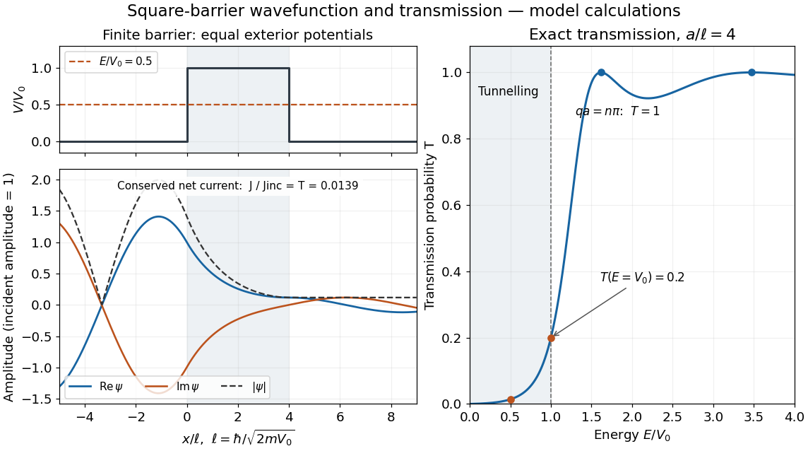
Matched square-barrier wavefunction and transmission below and above the barrier
. Original model calculations with equal exterior potential energies, constant mass and incident probability amplitude one. The real part and imaginary part of the wavefunction, its modulus and the exact transmission probability are shown; these curves are not measurements. The conserved net probability current is small but nonzero throughout the barrier. Details.For a thick rectangular barrier with equal exterior potentials, constant mass and , the exact matched transmission probability has the displayed limit when . The exponential is fixed by the evanescent action; the interface prefactor remains energy-dependent. A leading-exponential estimate can therefore differ by an order-one multiplier from the matched result.
For fixed and , the exact rectangular barrier transmission probability givesThis is the leading term of an asymptotic expansion: the wavefunction amplitude scale is , and the transmission probability scale is , with an interface prefactor. Increasing width by multiplies this approximation by . At fixed incident energy, increasing barrier height increases the tunnelling decay constant as ; heavier nonrelativistic particles also have stronger suppression. For the numerical example in rectangular barrier transmission probability, the approximation gives , compared with the exact .
The regime condition matters. Near at fixed width, tends to zero and the opaque barrier approximation fails; use the exact threshold value. For , expansion of the hyperbolic sine givesThis tends to one as at fixed , but the condition alone does not imply nearly perfect transmission if the remaining factor is large. At , use the oscillatory formula and its scattering resonances, rather than an exponential decay law.
A nonzero probability density inside a barrier does not by itself imply transport. In one dimension, the probability current of a wavefunction is . A single evanescent wave has , a real quantity, hence . This is what happens on the inaccessible side of a potential barrier extending to infinity with .[ref]
For the finite-barrier wavefunction , the cross terms instead giveThe relative quantum phase of the two probability amplitudes permits a nonzero, spatially constant probability current, even though neither exponential function separately carries it. The probability continuity equation gives for this stationary state. Matching the wavefunction and its derivative also makes continuous at both faces, soHere is the quantum reflection probability, and is the transmission probability. The net exterior probability current equals the interior probability current; it is not lost as the wavefunction decreases. A physical incident wave packet supplies finite total probability, while the stationary state describes the energy component used to compute its transmitted flux.
Tunneling through a controllable vacuum gap by Gerd Binnig and others made barrier width experimentally adjustable. Their apparatus used a pointed electrical conductor opposite a conducting plate, with fine positioning by piezoelectricity. Rubber-tube support and magnetic levitation above a cooled bowl exhibiting superconductivity suppressed vibrations; the junction itself remained near room temperature.[ref]
The readout was electrical resistance versus displacement at a fixed electric potential difference of 60 mV of either polarity. They observed an exponential function dependence spanning four orders of magnitude. Cleaning and better vacuum increased the inferred barrier from approximately 0.6-0.7 eV to 3.2 eV. Reproducible curves and the cleaning response argued against deforming contamination layers; an appropriate slope also helped exclude an ordinary conducting contact. The paper reports residual contamination, electronics-limited range and a jump attributed to release of thermal stress; its curve origins generally do not determine absolute gap widths.[ref]
Tunneling through a controllable vacuum gap by Gerd Binnig and others. p. 179, equation (1), Fig. 2 and accompanying control/limitation discussion
The ideal tunnel junction model explains the slope. At fixed small electric potential difference, fixed tip geometry and approximately unchanged density of states, take an effective barrier energy above the relevant electron states and approximate the current magnitude byThe coefficient includes the applied electric potential difference, available occupied and empty quantum states, and tip geometry. A single transmission probability is not an electric current: a junction combines contributions from many electron states in both directions, with the electric potential difference producing a net imbalance. Its tilted, material-dependent barrier is only approximated by the equal-exterior rectangular potential barrier; the exact single-particle formula above is not a complete junction model.
For the chosen model value electronvolts, . Increasing separation by multiplies by about , a reduction by about . The following diagram chooses solely for illustration; it contains no measured data and is not a fit to the 1982 curves.
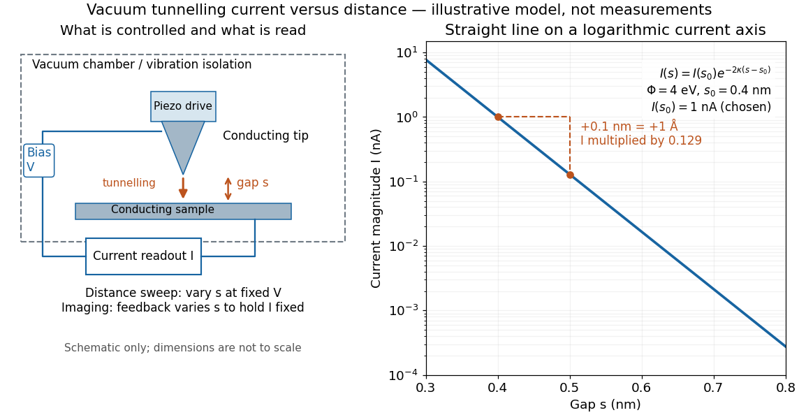
Distance calibration is essential. In Scanning Tunneling Microscopy: From Birth to Adolescence by Gerd Binnig and others, the authors describe an initial inferred barrier near 1 eV. Recalibration found only half the quoted piezo displacement sensitivity and raised the inferred barrier above 4 eV. Thus an exponential trace alone was insufficient evidence for tunnelling through vacuum. The model makes the sensitivity explicit: the inferred depends quadratically on the distance scale.[ref]
Scanning Tunneling Microscopy: From Birth to Adolescence by Gerd Binnig and others. p. 397, piezo-sensitivity calibration discussion
For scanning tunnelling microscopy, feedback control adjusts the vertical position to hold electric current fixed during a lateral scan; the recorded height follows separation only when the surface is electronically homogeneous. Changes in the local density of states can also change apparent height. This limitation is already explicit in the authors' account of constant-current imaging.[ref]
Scanning Tunneling Microscopy: From Birth to Adolescence by Gerd Binnig and others. p. 391, Fig. 2, joint local density of states; p. 396, Fig. 5(a), electronically homogeneous surface condition
The converse effect of piezoelectricity converts an applied electric potential difference into a small mechanical deformation, permitting fine control of a tunnel junction's separation.
A transducer using stress-induced electrical charge. A uniformly loaded slab of thickness has ideal open-circuit voltage sensitivity ; leakage and input capacitance change its measured response.
The change in output voltage per input stress under specified geometry, loading direction, frequency and electrical boundary conditions.
Linear electrical-displacement response to mechanical stress in a suitable piezoelectric material. It is distinct from the converse effect, in which an applied electric field causes strain. The measured voltage also depends on electrical loading and mechanical constraints.
For electrically isolated electrodes with unchanged free charge, the increment of normal electric displacement field is approximately zero. A constitutive relation such as then gives an induced field that balances stress-induced displacement. Finite leakage and input capacitance modify the voltage response.
A tensor coefficient relating an increment of electrical displacement to stress, or the corresponding converse strain response to electric field, under stated constitutive conventions. Charge-per-force units are equivalent to displacement-per-voltage units for the usual coefficients.
Dependence of piezoelectric displacement on the history and direction of the applied voltage. It differs from the continuing time-dependent relaxation called piezoelectric scanner creep.
Slow displacement relaxation following a change in piezoelectric scanner drive, even after the commanded voltage is held fixed. Settling and position-sensor closed-loop control reduce its effect on image coordinates.
Mechanical strain induced by an applied electric field. It complements the direct conversion of mechanical stress into electrical polarization.
A material exhibiting piezoelectricity, used in the Curie ionization-current measurement to supply a controlled electric charge.
A tunnel junction separates two conducting electrodes by a thin barrier through which electrons undergo quantum tunnelling.
The work function is the minimum energy needed to remove an electron from a solid to the nearby vacuum level. A junction's effective barrier need not equal either electrode's isolated work function.
Scanning tunneling microscopy uses a scanning tunneling microscope to map a surface from the electric current across a tunnel junction. In constant-current operation, feedback control adjusts the tip height to maintain a chosen electric current. The current-distance test of vacuum tunnelling explains the underlying distance sensitivity and its measurement limits.
The image records the response of a tunnel junction, rather than photographing chemical atoms. Its apparent height can reveal both surface structure and the local density of states; distinguishing them is part of interpreting the measurement.[ref]
Scanning Tunneling Microscopy: From Birth to Adolescence by Gerd Binnig and others. p. 391, Fig. 2; p. 396, Fig. 5
Controlled positioning or modification of individual surface atoms or molecules, including manipulation with a scanning probe. A weakly coupled imaging pass locates the adsorbate; stronger tip interaction or suitable excitation changes its motion or binding. Subsequent imaging checks the result. Temperature, substrate, tip state and atomic species determine the useful mechanism.
A deliberately assembled xenon-atom surface pattern illustrating controlled atomic manipulation. Don Eigler and Erhard Schweizer reported individual xenon positioning on single-crystal nickel at about in their 1990 paper.[ref]
Transferring an adsorbate between substrate and probe tip, allowing pickup, lateral repositioning and deposition at a selected site. Its feasibility depends on the tip and substrate binding landscapes and on the controlled excitation.
Moving a surface adsorbate between lateral positions by coupling it to a nearby scanning-probe tip and moving the tip parallel to the surface. Pulling, pushing and sliding depend on the competing tip–adsorbate and substrate interactions.
A conducting tip probes the energy-dependent local density of states by recording tunnel current versus applied bias, often measuring with a small bias modulation and lock-in detection. At low temperature and for slowly varying tip density and matrix element, is proportional to sample local density of states at the corresponding bias energy. Thermal broadening, surface structure and energy-dependent tunnelling selectivity limit a direct interpretation as bulk band structure.
Interference between incident and elastically reflected surface-state waves gives density oscillations proportional to . Their real-space period is , half the travelling-wave wavelength.
Low-temperature scanning tunneling spectroscopy resolves energy-dependent interference in the surface electronic density of states near scattering features. Its coexistence with a structural map distinguishes electronic corrugation from atomic positions. The 1993 Cu(111) observation provides an early example.
Vibrational excitation opens additional tunnelling channels at biases satisfying . A step in differential conductance gives paired opposite-sign features in its voltage derivative.
In the 1982 experiment, separate drives using piezoelectricity scanned a metal tip laterally and adjusted its height. A control unit held electric current fixed at constant tip-sample electric potential difference; calibrated drive voltages supplied the displacement readout. Their Fig. 1 explicitly contrasts a surface step with apparent height from contamination changing the work function.[ref]
Surface Studies by Scanning Tunneling Microscopy by Gerd Binnig and others. pp. 58–59, Fig. 1, equation (1), piezodrive calibration
Gerd Binnig and Heinrich Rohrer describe a later vibration isolation system using two spring stages and eddy current damping inside a vacuum chamber, with sputtering and annealing for surface preparation. These measures addressed unwanted motion and surface condition separately.[ref]
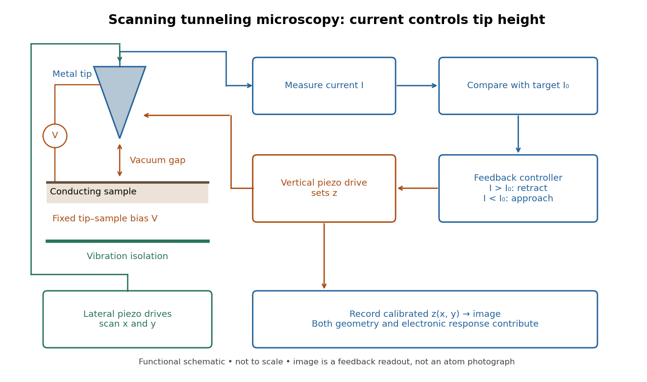
Choose a fixed tip-sample electric potential difference and a positive target electric current magnitude . At each lateral position , feedback control adjusts until the measured electric current approaches . Since increasing the gap reduces quantum tunnelling, excessive electric current calls for retraction; insufficient electric current calls for approach. The image is the calibrated vertical displacement , while the residual electric current error tests how closely the loop followed its target.
This is a contour of equal electric current, not necessarily a contour of equal separation. The electronic contrast in scanning tunneling microscopy model below shows why. It also explains the value of vibration isolation: an unintended displacement changes the same sensitive gap as the feature being measured. A scan must be slow enough for the finite bandwidth of feedback control; otherwise lags the desired contour.
Separate geometry from electronic response in an original one-dimensional toy tunnel junction. Write the geometric surface height as , tip height as , and positive gap as . Assume low fixed tip-sample electric potential difference: the sampled energy window is narrow enough that the tip density of states is featureless and the sample local density of states varies little across that window. Neglect thermal broadening, changes of tip shape and lateral averaging. Let be the effective sample local density of states divided by a positive reference value, so it is dimensionless. Choose a spatially constant effective barrier energy , a positive coefficient with units of electric current, andHere is the electron mass, the reduced Planck constant, and the tunnelling decay constant. This is an illustrative low-bias model, not a universal calibration formula. At fixed , taking a logarithm givesThe logarithms have dimensionless arguments. Only constant makes the recorded height differ from geometric height by a constant. Multiplying by raises the apparent height by without moving the geometric surface.
For a concrete ambiguity, choose , , lateral period , , and . CompareBoth produce exactly at . Substitution checks this without identifying with geometric height: case A has constant gap , while case B has gap and a compensating electronic factor. The chosen ranges from to , approximately to ; every gap remains positive. The chosen corresponds to electronvolts, a positive effective barrier.
At fixed tip height , both cases instead giveTheir maximum-to-minimum electric current ratio is . Thus even adding this fixed-height scan at the same electric potential difference cannot distinguish these deliberately chosen surfaces within the toy model. Independent structural information or additional electronic measurements are required. Changing electric potential difference can supply such information, but also changes the assumptions used to define and .
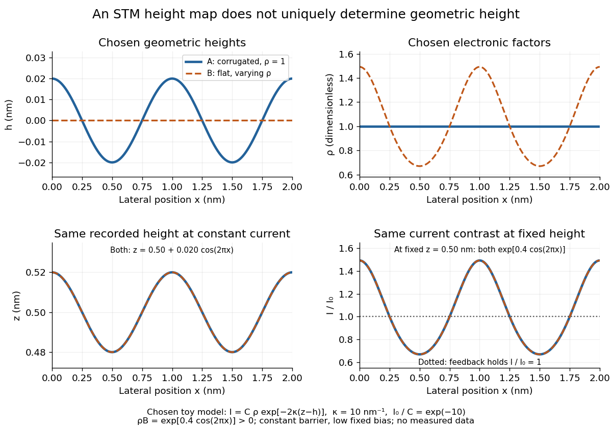
Different geometric and electronic profiles can produce the same STM image
. Original toy calculations, not measured data. The corrugated surface with constant local density of states and the flat surface with varying local density of states give identical recorded heights under constant-current scanning tunneling microscopy. They also give identical fixed-height electric current contrast at this chosen bias. Details.For gold (110), the 1982 paper compared an untreated surface with one prepared by argon sputtering and annealing. Repeated cleaning reproduced the corrugation; the gap-modulation signal checked work function variation. This supported a structural interpretation while exposing the danger of confusing work function contrast with geometric relief.[ref]
Surface Studies by Scanning Tunneling Microscopy by Gerd Binnig and others. p. 59, Au preparation, repeated cleaning and modulated signal
The authored lecture describes resolving the surface reconstruction on gold (110), alongside ribbons of other periodicities. It also reports gold transfer to the tip on contact and fluctuating resolution, attributed tentatively to migrating tip chemical atoms. The probe could change during observation: an image was evidence requiring controls, not an unambiguous map of atomic positions.[ref]
Scanning Tunneling Microscopy: From Birth to Adolescence by Gerd Binnig and others. pp. 398–399, Au(110) reconstruction, tip coating and changing resolution
A symmetric two-well system has nearly localized left/right states coupled by a positive quantum tunnelling magnitude . Its effective Hamiltonian is , so the superposition with an even spatial wavefunction is lower, and the level splitting is . The dilute instanton gas reproduces these two exponents through even/odd crossing sums.
For normalized localized states related by reflection and real overlap , the displayed superpositions are normalized even and odd states. The even state is lower for the lowest tunnelling pair; the odd state has one central node. Small overlap explains nearly identical probability densities in the two distant wells, but the relative phase remains different. A localized one-well state is a superposition of the pair rather than an exact stationary parity eigenstate.
For a square potential barrier of width and height , putThe oscillatory wavenumber outside and decay constant inside are both . Matching the wavefunction and its derivative at both faces gives transmission amplitudeand transmission probability .



