
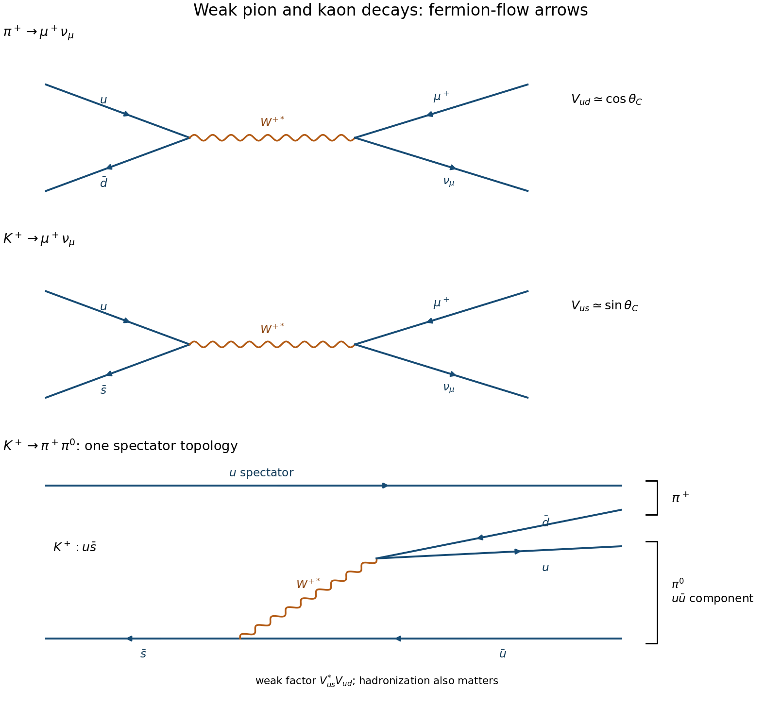
The charged meson decays proceed through a virtual :The first quark vertex has CKM factor , while the second has . In the simple Cabibbo description these are approximately and , so the strange amplitude carries a suppression relative to the nonstrange one, or in their corresponding squared weak-coupling factors.
For a charged pseudoscalar and a negligibly massive neutrino, the leading leptonic energy width has the formin natural units. The helicity factor is common to these two muon channels, while the threshold factor is much less favorable for the pion. Using the usual masses, its value is about for the pion and for the charged kaon: the pion's threshold factor alone is only about one fifth as large. Including the explicit factor gives a kinematic ratio about . The pseudoscalar decay constants also matter, so Lorentz-invariant phase space and CKM factors alone do not determine the full lifetime ratio.[ref]
Leptonic Decays of Charged Pseudoscalar Mesons by Particle Data Group. leading pseudoscalar leptonic-width formula and pion/kaon discussion
For , one tree topology has the spectator unchanged and followed by . The spectator can combine with to form , and the component supplies . This carries the strangeness-changing weak factor . Hadronization, other quark rearrangements and strong final-state interactions determine the hadronic amplitude; the diagram is not a complete precision width calculation. The small pion–muon energy release suppresses the pion leptonic channel kinematically, whereas the strange weak vertex suppresses the kaon channels through Cabibbo suppression.

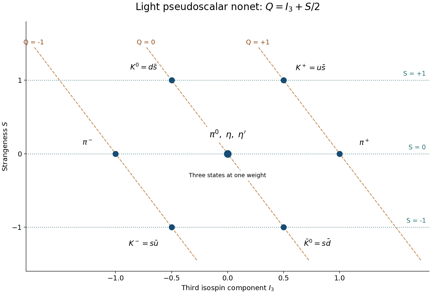
The light pseudoscalar meson nonet has and flavor structure . Its members are the three pions, four kaons, and the two neutral isospin-zero states eta meson and eta prime meson. For mesons the baryon number is zero, so the Gell-Mann--Nishijima formula reduces toHere is strangeness, with an quark carrying and an antiquark carrying . Thus the upper row is at and at . The lower row is at and at . The charged pions lie at , while share as flavor-weight coordinates.
The neutral pion direction is . The octet and singlet isoscalar directions mix to make the physical eta and eta-prime states; counting three central states is essential to obtaining nine rather than seven particles. Horizontal lines in the diagram have constant , while lines mark constant charge. Meson exchange describes part of the residual nuclear force; the underlying quark-level strong interaction is mediated by gluons, not by treating pions as elementary gauge bosons.

For exponential decay with mean lifetime , the state amplitude evolves as and its survival probability is . Hence the energy decay width isThe exceptionally small energy width expresses the long lifetime of this weak decay. Use , not , because is an energy width in the complex-energy convention; changing to a frequency convention introduces the appropriate factor of . The quoted lifetime is treated as the mean lifetime. If a half-life were supplied instead, one would first use . No extra logarithm is needed for the given mean-lifetime interpretation. This calculation uses the source's approximate 15-minute value rather than silently replacing it with a more precise contemporary neutron-lifetime measurement.
Work first in units . In the neutron rest frame, let . From ,The electron's minimum possible total energy is its rest energy. This configuration has the electron at rest while the proton and massless antineutrino move back to back with equal momentum magnitudes. Their common momentum satisfies a two-body energy balance for the remaining mass :For the maximum electron energy, minimize . Since the massless antineutrino has nonnegative energy, , with the boundary reached as its energy tends to zero. ThenAt this limiting endpoint the electron and proton have equal and opposite momenta. The proton recoils; it is not at rest. A massless neutrino has no rest frame, so “neutrino at rest” must be replaced by the precise soft-energy limit . The electron's maximum kinetic energy is the displayed total energy minus , rather than the same number. These endpoint configurations lie on phase-space boundaries; their kinematic existence does not imply a nonzero event density exactly at the boundary.
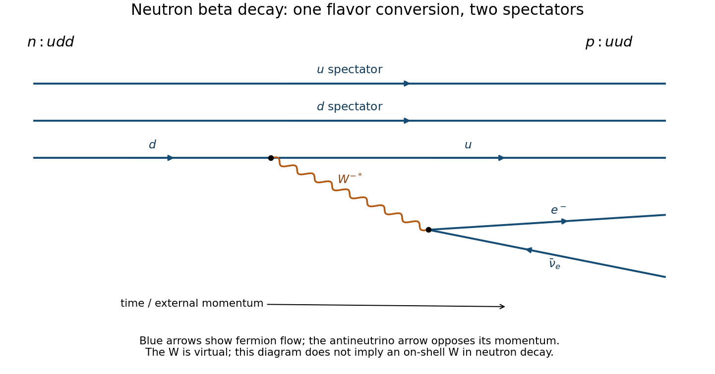
The charged weak current changes one neutron down quark into an up quark:The other two valence quarks are spectators in this tree-level Feynman diagram. The intermediate W boson is highly virtual; the available neutron decay energy is far below its on-shell rest energy. Charge is conserved at each vertex, and the electron's lepton number is balanced by the electron antineutrino.
The reversed quark-level charged current is allowed as an interaction, but a free proton cannot decay as because . Four-momentum conservation leaves no accessible final-state Lorentz-invariant phase space. The absence of this free-proton beta-plus decay is therefore kinematic, not an absence of a weak vertex. Binding-energy differences in a nucleus, or incoming energy in a collision, can change whether the corresponding conversion is possible. Exotic baryon-number-violating proton decay is a separate question and is not generated by this ordinary charged-current diagram.

Past exam of the sub-atomic physics course of the University of Oxford 2016 1 a Solution Created 2026-10-25 Updated 2026-11-05
The neutron has valence content and total spin ; its ground-state parity is positive. The two down quarks contribute charge and the up quark contributes , giving net charge zero. “Three valence quarks” specifies the net flavor quantum numbers, rather than excluding gluons or additional sea quark–antiquark components from the full quantum chromodynamics state.
In the approximate light-flavor SU(3) classification, the neutron belongs to the ground-state baryon octet, containing eight hadrons:These are eight particle species, without counting their antiparticles again as extra members of the same octet. The corresponding antibaryons form the conjugate particle set. Within the smaller SU(2) isospin classification, the neutron instead belongs to the two-member nucleon doublet . Stating the symmetry distinguishes the usual eight-member flavor multiplet answer from the also valid two-member isospin multiplet. The baryon decuplet has different ground-state spin and is not the neutron's octet.
For , , , the friction memory kernel and its Laplace transform areUsing the generalized fluctuation-dissipation relation with equilibrium velocity variance , the velocity autocorrelation function has Laplace transformAll three poles are negative, so the stationary relaxation is stable. A partial fraction decomposition givesTaking the inverse Laplace transform givesThe negative middle coefficient is compatible with an autocorrelation function; individual terms in a partial fraction decomposition need not themselves be separate physical modes with positive weights. Several useful checks follow directly:The Volterra integral equation for predicts exactly and . Its integral is also , agreeing with the Green-Kubo formula for diffusion.
We use the equilibrium generalized Langevin equation and its generalized fluctuation-dissipation relation, with the factor in the noise autocorrelation fixing the equilibrium velocity variance. Let be the velocity relaxation function and let a tilde denote a one-sided Laplace transform:The equilibrium velocity autocorrelation function is , soFor completeness, this relation follows without assuming independence of the noise and velocity in a stationary infinite history. The two-sided noise power spectral density is . The stable linear equation has velocity transfer function , soThis is precisely the power spectral density of the even extension of . Stable relaxation removes initial transients with a finite second moment, giving the long-time autocorrelation function defined in the question. All the parameter choices used below have stable relaxation.
Integrating the velocity autocorrelation function twice gives the mean squared displacement from a fixed initial position:A decaying initial transient does not change its asymptotic slope. Therefore the Green-Kubo formula for diffusion givesFor the given friction memory kernel, direct integration yieldsAt , the integrated friction is , henceThe relaxation denominator here is . Its roots have negative real parts by the cubic Routh-Hurwitz criterion, since all coefficients are positive and . This justifies the decay and integrability used above. The diffusion coefficient depends on the area under the friction memory kernel, not just its value at zero.
For a radial function in three dimensions, the Laplacian is , while the imposed radial drift contributes . Thus the radial generator of an SDE diffusion isThe hitting probability for the inner sphere is harmonic for this diffusion generator in the shell, with value one on the inner sphere and zero on the outer sphere. At , the boundary value problem is thereforeIntegrating gives . The two boundary conditions determineBoth arguments of the logarithms are dimensionless. The result decreases from one to zero across the shell and lies strictly between zero and one for .
For a direct probability interpretation, stop at the first contact with either sphere. The stopped process is a bounded martingale by Itô's formula. The shell has positive inner radius, so its drift is bounded and its diffusion is nondegenerate; exit occurs almost surely. Optional stopping and dominated convergence therefore giveThe logarithm appears because the inward drift cancels one of the two geometric terms in the three-dimensional radial Laplacian, leaving the same radial diffusion generator as a planar Brownian motion with diffusion coefficient one.
At the transverse coordinates are independent Brownian motions with diffusion coefficient . The cylinder is infinitely long, so the axial coordinate cannot affect its first contact time. By rotational invariance of Brownian motion, the mean first-passage time depends only on the transverse radius .
The Kolmogorov backward equation for a mean first-passage time is . Here , so the radial boundary value problem isThe absorbing boundary condition for a diffusion is imposed on the circular cross-section. At , the solution must extend smoothly over the axis. Multiplying by and integrating givesSmoothness at the axis excludes the logarithm term, and fixes . ConsequentlyThis also verifies the finiteness assumption behind the Kolmogorov backward equation. Let be the first contact time and apply the stopped Itô formula to the bounded nonnegative function just obtained. Its bounded derivatives on the disk make the stopped stochastic integral a martingale, givingBy monotone convergence, has finite expected value; continuity and dominated convergence then make the final term vanish as . Hence . In particular, the mean first-passage time is on the axis and tends to zero at the adsorbing wall.
The native PDF repeats in its list of independent noise terms, whereas its third stochastic differential equation uses . We use the intended three independent coordinate Brownian motions .
Put , and . Before the origin is reached, Itô's formula givesThe is the sum of three quadratic variation terms, each . The drift contribution is because the numerator is . The radial stochastic integral can be written using a scalar Brownian motion :Thus is a squared Bessel process of dimension until it reaches zero. If this equation is taken globally with the usual nonnegative squared Bessel process continuation, taking expected values givesThe stochastic integral has zero expected value: stopping first at large levels bounds the integrands, yields a finite first moment for , and then makes finite, so the unrestricted integral is a square-integrable martingale.
Boundary qualification. The punctured domain in the question does not itself specify that continuation. The boundary classification of a Bessel process says that the origin is inaccessible from when , equivalently . In this parameter range the original stochastic differential equation is global in the stated domain and the boxed result holds as written.
For , we have : the origin is reached in finite time with probability one. One can also see accessibility directly from the radial generator of an SDE diffusionFor , the harmonic function is the probability of reaching zero before . Finite-time access follows by using the nonnegative functionin the stopped Itô formula; it bounds the expected value of the time to reach zero or . Letting gives almost sure finite hitting of zero. The coefficients of the original vector stochastic differential equation are undefined there, so its stated punctured-domain version has no prescribed long-time evolution in this range.
The natural continuing radial squared Bessel process gives , but stopping and holding the particle at the origin would give a different answer. Indeed, with the first hit of zero, Itô's formula for the stopped process givesSince almost surely, dominated convergence applied to givesTherefore is the usual continued-radial answer; for a boundary convention is necessary. It is not a uniquely defined limit for the punctured-domain model alone.
A product-Poisson stationary distribution is suggested by balancing the three reaction fluxes around the directed cycle of reaction complexes. If their mean counts are , this complex balance condition iswhich gives and . This suggests the joint probability mass functionIt is normalized because it is the product of two Poisson distributions. We verify it directly in the chemical master equation, rather than assuming a product-Poisson stationary distribution theorem. The three incoming terms satisfyWith negative-index values set to zero, these identities also hold on the axes. Their sum equals , precisely the outgoing probability flux. The stationary average total exit rate is , so these stationary balance equations do define an invariant distribution of a continuous-time Markov chain for the nonexplosive model verified below. This is complex balance; it does not assert pairwise detailed balance for the irreversible chemical reactions.
To identify this invariant distribution with the limiting probability distribution in the question, first check that the model is a nonexplosive continuous-time Markov chain. On any finite time interval, is bounded by its initial count plus the finite number of arrivals in a rate- Poisson process. Conditional on that bound, the rate of producing is bounded, so only finitely many such productions occur. The number of joint removals cannot exceed the available molecules. Thus only finitely many chemical reactions occur in finite time.
The continuous-time Markov chain is also an irreducible Markov chain. From a Markov chain state with both counts positive, repeated joint removals reduce both. On the axis, producing one and then removing a pair reduces by one. On the axis, adding one and then removing a pair reduces by one. Each prescribed finite sequence has positive probability, so every Markov chain state reaches . Conversely, arrivals followed by productions reach any with ; to reach , reach and remove one pair. The continuous-time Markov chain is therefore positive recurrent, and the continuous-time Markov chain convergence theorem gives from the empty initial condition.
Conditioning on the observed time. The native PDF defines as the first production time and then conditions on that production occurring at . If the intended information is its numerical value , the answer depends on . We first compute this conditional probability using a conditional probability density; conditioning on an exact value of a continuous random variable means a density ratio, since .
Before , no molecules of the second chemical species are present, so the joint-removal chemical reaction cannot occur. Molecules of the first chemical species arrive as a rate- Poisson process, and each independently starts a clock with a rate- exponential distribution for producing the first molecule of the second chemical species. Define the unnormalized probability mass functionThe chemical master equation before the first production, with production treated as killing, isMultiplying by and summing gives a partial differential equation for the probability generating function:Its solution, verifiable by direct differentiation, isThus , the survival function is , and the conditional distribution of given survival to is a Poisson distribution of mean .
Production in from Markov chain state has joint probability . Therefore the probability density function of isThe first production leaves unchanged. Taking the density ratio gives a size-biased distribution of the surviving count:In particular, under this reading the requested conditional probability isThe shift by one matters: an observation made exactly when production occurs preferentially selects larger counts, since their production reaction propensity function is larger.
Without observing the numerical time. If the conditioning merely repeats the definition of , the requested probability is instead the unconditional count at that stopping time. Before production, increases by one at rate , while production occurs at rate in Markov chain state . The competing exponential clocks implyThe first factor requires a second arrival before production from count one; the second requires production before a third arrival. The first arrival itself is certain. Production eventually occurs with probability one, as is also clear from . As a consistency check, averaging the time-conditioned answer against givesThese are two distinct, explicitly specified interpretations of the printed conditioning.
There are unlisted articles, also show them or only show them.