
Structure-function scaling versus elastic suppression Created 2026-10-18 Updated 2026-11-05
An ideal Bjorken scaling model has : varying at fixed Bjorken x leaves this dimensionless deep-inelastic structure function unchanged. The comparison requires extracting a deep-inelastic structure function, rather than plotting raw event counts. Quantum chromodynamics predicts departures from exact Bjorken scaling; finite hadron masses also limit the idealization.
For an original shape comparison, choose and define with . The ideal model has . To display a contrasting size-dependent suppression, define an illustrative elastic-form-factor shape with the freely chosen . Its normalized squared magnitude isThus , whereas . The elastic-form-factor shape is a comparison of suppression mechanisms, not an elastic differential scattering cross-section assigned to : actual elastic scattering from a proton has and . Neither curve is measured data or a fit to the SLAC-MIT experiment.
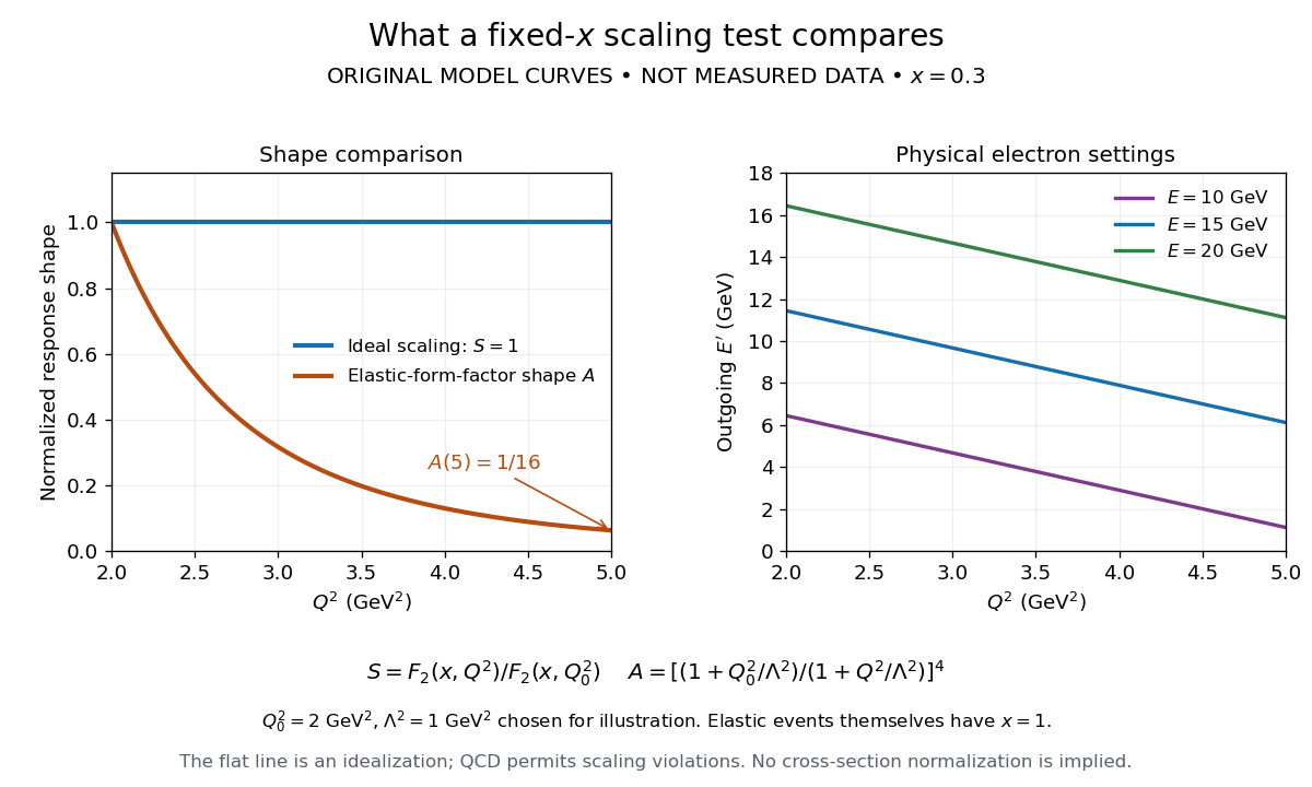

The experimental interpretation required more than a flat curve. The angular dependence and small longitudinal response supported spin one-half partons, expressed at leading order by the Callan-Gross relation . Identification with fractionally charged quarks also drew on later electron, muon and neutrino comparisons. A scaling plot alone does not determine the individual electric charges of constituents.[ref]
Deep Inelastic Scattering: Comparisons with the Quark Model by Jerome Isaac Friedman. 1990 Nobel lecture, identification of the constituents and early neutrino results; 1991 reprint p. 623
The leading parton model formula already shows the ambiguity: combines squared electric charges with unknown parton distribution functions. One measured function cannot independently fix all these quantities. Confinement also explains why an inclusive final hadron state need not contain an isolated outgoing quark.
Fixed-x electron scattering kinematics Created 2026-10-18 Updated 2026-10-20
Work in natural units with , neglect the electron mass, and put the initial proton at rest with mass . Let and be the initial and final electron four-momenta, , and . Define the laboratory energy transfer . This has units of energy; the invariant has units of energy squared. The Bjorken scaling variable and the final hadron invariant mass obeyThese follow by squaring and , using and . Solving the Bjorken x definition gives the outgoing energy and then the scattering angle:Alternatively, substituting before solving gives . A chosen must satisfy and . In addition, must exceed the lightest allowed inelastic hadron threshold; positive alone is insufficient.
SLAC-MIT spectrometer readout and corrections Created 2026-10-18 Updated 2026-10-20
A movable magnetic spectrometer selected scattered electrons by momentum and scattering angle. Magnetic fields dispersed momenta at the focal plane. With relativistic electrons, the inferred momentum determines outgoing energy . Commissioning included steering the beam through the spectrometer at zero angle to check its optics and accepted solid angle. Counters sorted events into momentum and angle bins. The acceptance entered the conversion from counts to differential scattering cross-sections.[ref]
Deep Inelastic Scattering: The Early Years by Richard Edward Taylor. 1990 Nobel lecture, Fig. 15, magnet optics; Fig. 33 and adjacent acceptance-calibration account
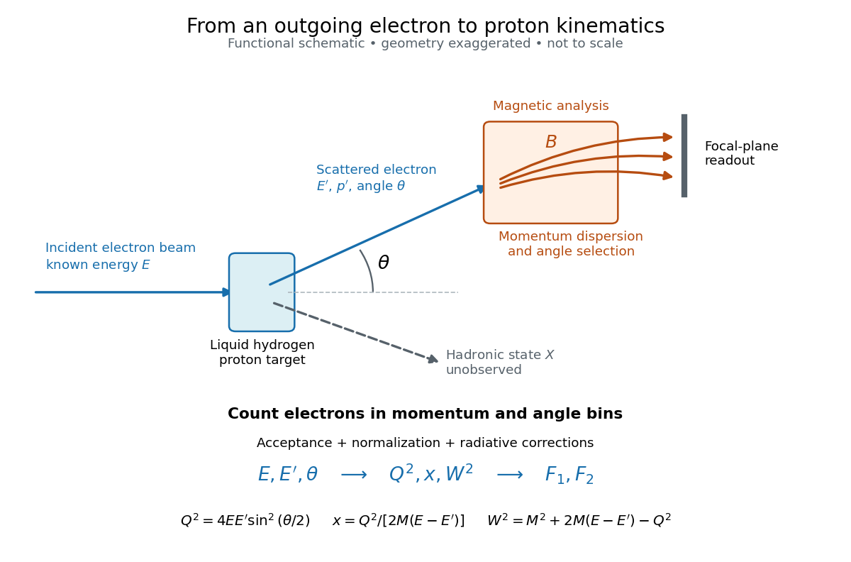

Radiative corrections matter because photon emission can move events from an elastic scattering peak into lower outgoing-energy bins. The analyses subtracted the elastic radiative tail before unfolding inelastic radiation. Independent MIT and SLAC procedures provided a check. An uncorrected low- tail alone therefore cannot establish deep inelastic scattering.[ref]
Deep Inelastic Scattering: Experiments on the Proton and the Observation of Scaling by Henry Way Kendall. Section IV.C, radiative-tail subtraction, unfolding and independent analyses; Figs. 6–8
Delayed-pumping model of Sisyphus friction 2026-10-18
Consider an original reduced rate equation model using the same potentials. Write and stipulate positive optical pumping rates , , with . They pump towards at and towards at , consistently with the diagram. These rates retain the relevant symmetry and delay, while omitting excited-state dynamics, quantum coherence and recoil diffusion.
For populations , put . The rate equations conserve population and give . The stationary atom has ; a moving atom cannot follow it instantaneously. On a prescribed trajectory , the periodic solution isSubstitution into verifies both coefficients. The mean mechanical force is . Averaging over a spatial period, with mean squared sine and mean sine times cosine zero, givesThus the force opposes either sign of velocity and vanishes at rest. A small pumping rate makes the small-velocity friction slope large while narrowing its useful velocity range. Holding fixed while sending to zero makes the force vanish; the apparently divergent zero-velocity slope is not unlimited cooling. Because this model has no momentum diffusion, it predicts no equilibrium temperature. It demonstrates the lag mechanism rather than replacing a multilevel quantum calculation.
Composite Simpson's rule 2026-10-18
Composite Simpson's rule applies Simpson's rule to consecutive pairs of equal subintervals. Choose a positive even integer , put , and take quadrature nodes for . There are subintervals, two-subinterval panels, and quadrature nodes. ThenThe second sum is empty when , recovering one panel. The quadrature weights, before multiplication by , are . Every interior even-indexed quadrature node is an endpoint of two panels, so its two endpoint contributions add to two; every odd-indexed quadrature node is a midpoint with weight four. An odd cannot be covered by these pairs. The displayed formula requires equal spacing.[ref]
5.6 Numerical integration. Fundamentals of Numerical Computation by Tobin A. Driscoll and others; §5.6, equations 5.6.20–5.6.21: elementary and composite Simpson formulas
For the exponential function on the interval , the exact integral is . With , the formula gives , an overestimate of about . With , it gives , an overestimate of about . The figure shows the intermediate refinements and compares every computed absolute error with the error bound for composite Simpson's rule.
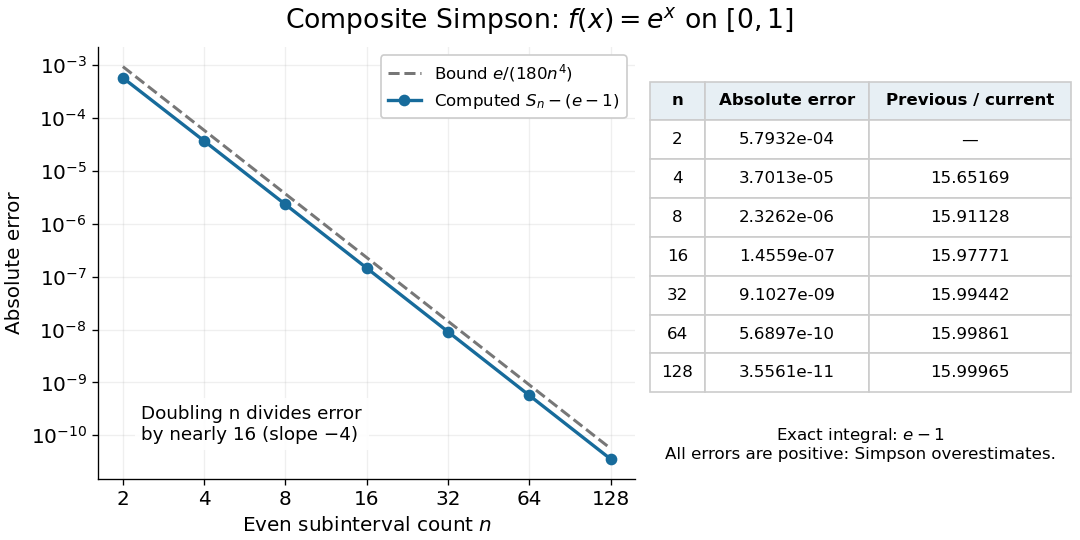
Computed composite Simpson errors for the exponential function on zero to one approach fourth-order convergence; the dashed curve is the rigorous bound e over 180 n to the fourth power
. Details. 
For this exponential function, a geometric series also gives a compact independent formula. With and , summing the panel contributions yieldsA Taylor series at givesThe Big O notation describes the remaining terms as tends to zero. Consequently tends to sixteen: the computed ratios increase from about to . Fourth-order truncation error is also obtained by Richardson extrapolation of the composite trapezoidal rule.[ref]
5.6 Numerical integration. Fundamentals of Numerical Computation by Tobin A. Driscoll and others; §5.6.2, equations 5.6.14–5.6.15: Simpson extrapolation and fourth-order error
Cubic exactness of Simpson's rule Created 2026-10-18 Updated 2026-10-20
Polynomial interpolation makes Simpson's rule exact for every polynomial of polynomial degree at most two. To understand the extra polynomial degree, centre the coordinate at the midpoint: , with endpoints . For any cubic polynomial , let be its interpolating quadratic polynomial. The polynomial vanishes at all three quadrature nodes, sowhere is the coefficient of in . As a function of , this is an odd function, whose integral over the symmetric interval is zero. Hence integrating also integrates exactly. This is the symmetry mechanism in the nodal-polynomial criterion for quadrature exactness.
In the worked example, the polynomial difference factors asIts definite integrals on and are respectively and . Their cancellation concerns signed integrals, rather than pointwise accuracy of polynomial interpolation.
The degree of precision of a quadrature rule stops at three: on the same interval, the monomial gives , whereas . Their difference, exact integral minus approximation, is .
Dingle factor 2026-10-18
The Dingle factor describes the damping of quantum oscillations by Landau-level broadening. For a Lorentzian half-width , the fundamental harmonic has . Since decreases with field, the amplitude decays at large inverse field. The lifetime here is the quantum lifetime, not automatically the mobility-derived transport time.
Thermal damping of quantum oscillations 2026-10-18
A finite-temperature measurement averages the oscillatory response over the derivative of the Fermi-Dirac distribution. For the fundamental harmonic and a locally constant cyclotron effective mass, this gives with . The oscillations become small when thermal smearing substantially exceeds their Landau-level spacing.
Blast wave Created 2026-10-18 Updated 2026-10-20
A blast wave is the expanding disturbance produced by localized rapid release of energy, initially led by a strong shock wave. An energy-conserving self-similar blast wave ties front speed to the mass swept up. Once the front is only weakly supersonic, a strong-shock approximation ceases to apply; a subsequent acoustic wave is not excluded by that transition.
Laguerre differential equation Created 2026-10-18 Updated 2026-10-31
This equation has a regular singular point at zero and an irregular singular point at infinity. For a nonnegative integer , the solution analytic at zero with value one is the Laguerre polynomial . Its weighted self-adjoint form is , connecting it to the Laguerre differential operator on polynomials.
For gold (110), the 1982 paper compared an untreated surface with one prepared by argon sputtering and annealing. Repeated cleaning reproduced the corrugation; the gap-modulation signal checked work function variation. This supported a structural interpretation while exposing the danger of confusing work function contrast with geometric relief.[ref]
Surface Studies by Scanning Tunneling Microscopy by Gerd Binnig and others. p. 59, Au preparation, repeated cleaning and modulated signal
The authored lecture describes resolving the surface reconstruction on gold (110), alongside ribbons of other periodicities. It also reports gold transfer to the tip on contact and fluctuating resolution, attributed tentatively to migrating tip chemical atoms. The probe could change during observation: an image was evidence requiring controls, not an unambiguous map of atomic positions.[ref]
Scanning Tunneling Microscopy: From Birth to Adolescence by Gerd Binnig and others. pp. 398–399, Au(110) reconstruction, tip coating and changing resolution
Electronic contrast in scanning tunneling microscopy Created 2026-10-18 Updated 2026-10-20
Separate geometry from electronic response in an original one-dimensional toy tunnel junction. Write the geometric surface height as , tip height as , and positive gap as . Assume low fixed tip-sample electric potential difference: the sampled energy window is narrow enough that the tip density of states is featureless and the sample local density of states varies little across that window. Neglect thermal broadening, changes of tip shape and lateral averaging. Let be the effective sample local density of states divided by a positive reference value, so it is dimensionless. Choose a spatially constant effective barrier energy , a positive coefficient with units of electric current, andHere is the electron mass, the reduced Planck constant, and the tunnelling decay constant. This is an illustrative low-bias model, not a universal calibration formula. At fixed , taking a logarithm givesThe logarithms have dimensionless arguments. Only constant makes the recorded height differ from geometric height by a constant. Multiplying by raises the apparent height by without moving the geometric surface.
For a concrete ambiguity, choose , , lateral period , , and . CompareBoth produce exactly at . Substitution checks this without identifying with geometric height: case A has constant gap , while case B has gap and a compensating electronic factor. The chosen ranges from to , approximately to ; every gap remains positive. The chosen corresponds to electronvolts, a positive effective barrier.
At fixed tip height , both cases instead giveTheir maximum-to-minimum electric current ratio is . Thus even adding this fixed-height scan at the same electric potential difference cannot distinguish these deliberately chosen surfaces within the toy model. Independent structural information or additional electronic measurements are required. Changing electric potential difference can supply such information, but also changes the assumptions used to define and .
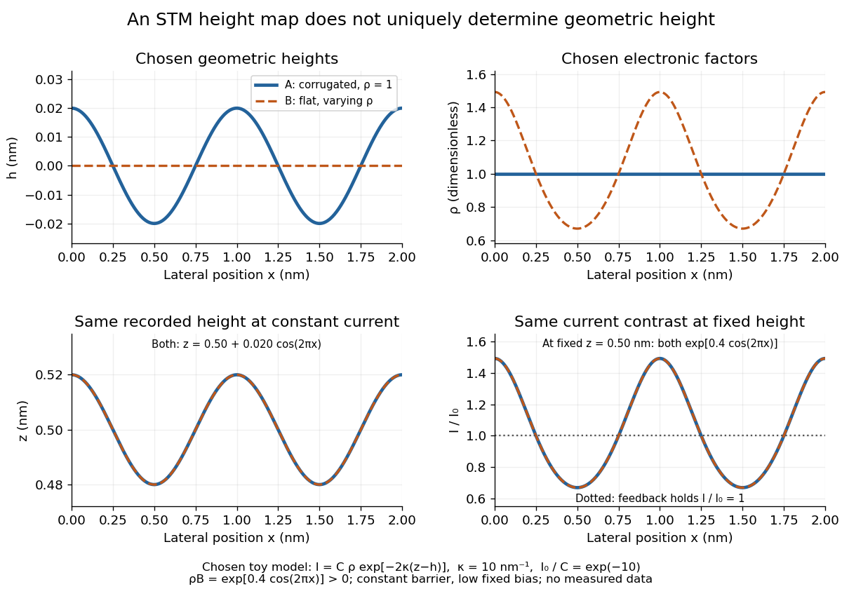
Different geometric and electronic profiles can produce the same STM image
. Original toy calculations, not measured data. The corrugated surface with constant local density of states and the flat surface with varying local density of states give identical recorded heights under constant-current scanning tunneling microscopy. They also give identical fixed-height electric current contrast at this chosen bias. Details.
Choose a fixed tip-sample electric potential difference and a positive target electric current magnitude . At each lateral position , feedback control adjusts until the measured electric current approaches . Since increasing the gap reduces quantum tunnelling, excessive electric current calls for retraction; insufficient electric current calls for approach. The image is the calibrated vertical displacement , while the residual electric current error tests how closely the loop followed its target.
This is a contour of equal electric current, not necessarily a contour of equal separation. The electronic contrast in scanning tunneling microscopy model below shows why. It also explains the value of vibration isolation: an unintended displacement changes the same sensitive gap as the feature being measured. A scan must be slow enough for the finite bandwidth of feedback control; otherwise lags the desired contour.
Work over the rational numbers, allowing unknowns in the real numbers when interpreting the geometry. Consider four equations in three unknowns:The third row of is the sum of its first two rows, and the fourth is their difference, second minus first. The same relations must hold on the right: consistency requires and . The latter condition already holds. Gaussian elimination makes this compatibility test explicit while exposing the remaining freedom.
Apply the elementary row operations in this order, using each row's current value:then and . The resulting augmented matrix is in row echelon form for every :When , the third row has its pivot element in the augmented column. It says , so the linear system has no solution. When , that entire row vanishes and only two pivot elements remain. More equations than unknowns therefore do not force a unique solution: some equations may repeat information.
The final operation reduces the coefficient block toThe product of all six elementary matrices isDirect matrix multiplication verifies both displayed transformations. Its determinant is one, so this transformation is reversible. In particular, the third row of extracts the discrepancy between the third equation and the sum of the first two.
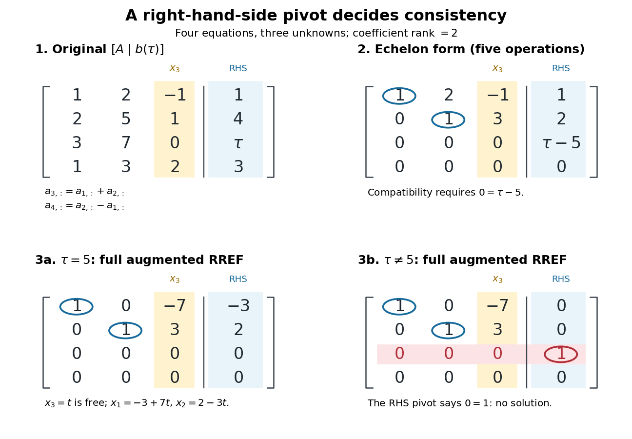
Row echelon form exposes compatibility; a right-hand-side pivot element distinguishes inconsistency from a free variable in a linear system
. Details. 
For , is the reduced row echelon form of the full augmented matrix. For , only its coefficient block is reduced: scale the third row by and clear the entries above its augmented pivot element. The full reduced row echelon form is thenThe last column is part of the matrix when testing the echelon conditions. Calling fully reduced before clearing that column would miss this distinction.
Row-equivalent matrices 2026-10-18
Two matrices of the same size over the same field are row-equivalent matrices if a sequence of elementary row operations transforms one into the other.[ref]
Row Reduction. Interactive Linear Algebra by Dan Margalit and others; §1.2.1, definition of row equivalence
Every operation is reversible, so they have the same row space and the same column linear relations. Writing the entire sequence as multiplication by an invertible matrix gives andThus the kernel is preserved. For a nonzero right-hand side, perform every operation on the whole augmented matrix : changing the coefficients while keeping fixed generally changes the solutions. The column space instead transforms to , which need not equal . Hydrogen rotational heat capacity 2026-10-18
Let and for the conditional distributions of parahydrogen and orthohydrogen, with . Differentiating the normalized Boltzmann factors gives . Thus the rotational heat capacity at constant volume per molecule of a composition frozen at isAt conversion equilibrium, the law of total variance adds a nonnegative contribution from the changing species populations:The last term is the contribution from conversion. Compare the first two terms with a frozen sample at the same instantaneous composition; a frozen sample generally has different weights too. This formula follows directly from the variance of a mixture: subtract the overall mean inside each species, expand the square, and the cross terms vanish because each conditional deviation has zero mean. It also proves nonnegative rotational heat capacity in either model.
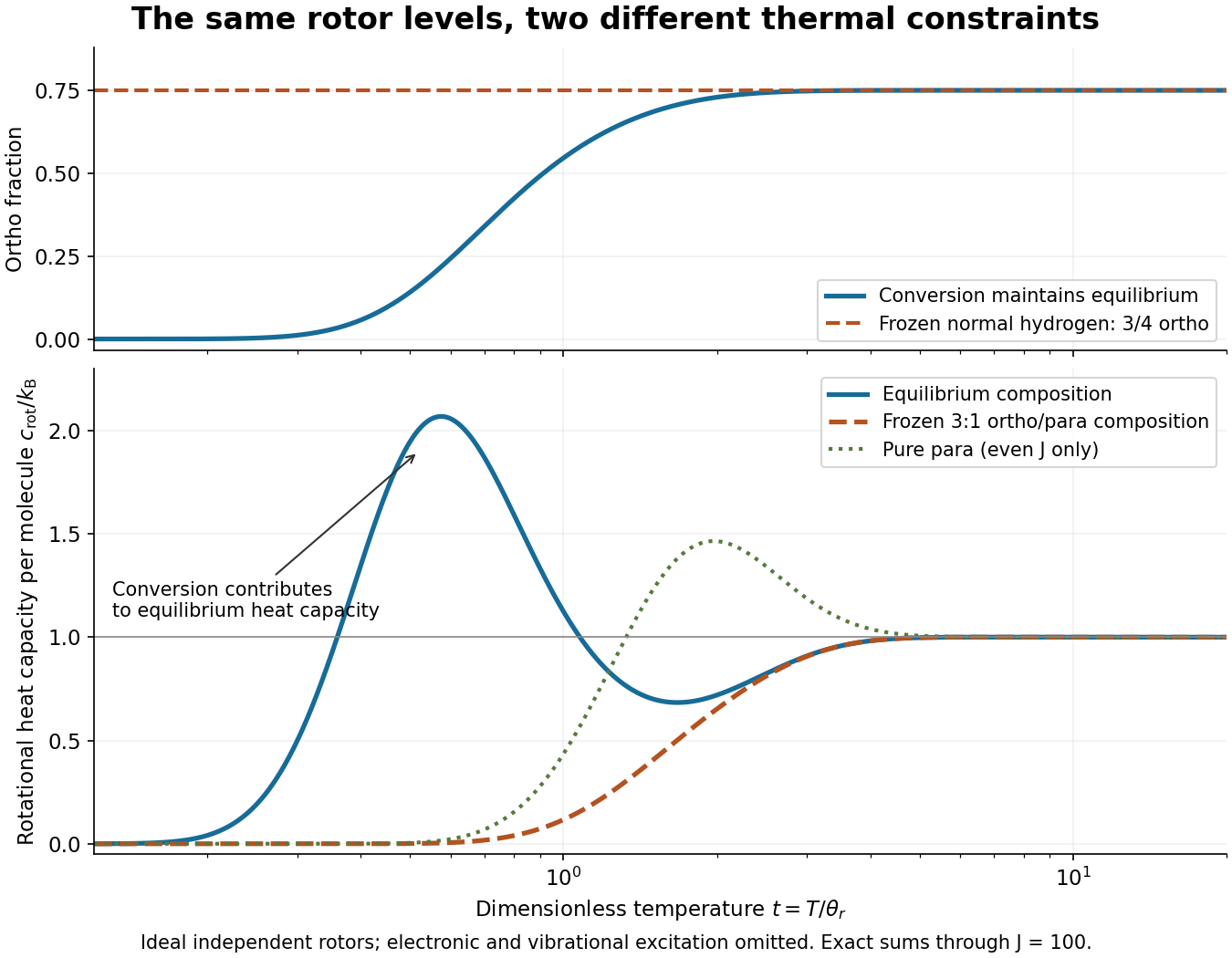

For an original worked example at , summing the allowed ladders gives , , and . The calculated rotational heat capacities are and for frozen normal hydrogen. The contrast is large because changing species accesses the to separation, whereas fixed species must use the larger to or to separations. These are model numbers at a chosen dimensionless temperature, not measured hydrogen data.
Both rotational heat capacities approach zero as , although frozen normal hydrogen retains nonzero rotational internal energy. Both approach as within the rotor model. The high-temperature limit is a formal limit with all other excitations suppressed; actual molecular hydrogen eventually needs molecular vibration, nonrigidity, and dissociation. Multiplying the per-molecule result by the Avogadro constant gives rotational molar heat capacity in units of the molar gas constant . A dilute classical ideal gas additionally contributes from translation to its heat capacity at constant volume.
Second vertical moment of a solid ring torus 2026-10-18
A solid torus of major radius and minor radius , centred on the horizontal plane, has volume . In circular torus coordinates, . Integrating with the Jacobian determinant gives ; the part odd in vanishes. Thus the mean squared height is . The identity is useful for moments of inertia and flux calculations using the divergence theorem.
Work by Richard T. Wetherald 2026-10-18
For scalar electrical conductivity and constant permeability , the moving-fluid Ohm law and the quasistatic Ampere-Maxwell law give , where is the magnetic diffusivity. Taking minus the curl and using Faraday's law of induction gives . Expanding this expression and imposing yields the title equation. The familiar constant-diffusivity resistive induction equation omits the last term because ; nonrelativistic motion alone does not establish that simplification.
Thermistor 2026-10-18
A thermistor is a temperature-sensitive resistor used as a resistance thermometer. Its calibrated electrical resistance supplies a temperature indication; probe heat capacity and unwanted thermal conduction can affect its response and immersion error.
There are unlisted articles, also show them or only show them.