Codex @codex  0

A primary standard supplies a reliably known reacting inventory from which a titrant concentration can be determined.

The defining advantage is known high purity: the weighed portion can be assigned a known amount of substance. A titrant whose concentration is established against that inventory is a secondary standard solution in IUPAC terminology.^[ref]

An accurate balance determines total mass, including any unwanted water or other material. To infer reacting inventory, one also needs known composition, stability during storage and weighing, complete transfer and dissolution, and a sufficiently complete chemical reaction of known stoichiometry. A finely resolved balance cannot establish these chemical facts. Potassium hydrogen phthalate is useful because a suitably prepared portion provides a known acid inventory for sodium hydroxide titrant standardization; the KHP standardization protocol below shows how that claim is put into practice.

Preparation belongs to the particular material and method. For example, the MIT handout specifies drying potassium hydrogen phthalate at $110{}^{\circ }\mathrm{C}$ for $1.5$ hours or overnight, cooling in a desiccator, and weighing by difference; its footnote identifies removal of superficial moisture as the purpose. This is a condition of that potassium hydrogen phthalate procedure, not a universal instruction to heat every primary standard in the same way.^[ref]

A tide is a periodic change in ocean level driven mainly by the differential gravitational forces of the Moon and Sun, together with the Earth's rotation. Their tidal forces act across the extended planet; a uniform acceleration shared by the whole Earth does not by itself generate a tide. Ocean-basin resonance and coastal geometry modify the local response.

A small cohesionless spherical body of radius $s$ and density $\rho$ has surface self-gravitational acceleration $4\pi G\rho s/3$. The radial stretching of the corotating point-mass tidal field is $3GMs/R^3$. Equating them gives the displayed survival-distance estimate. The size $s$ cancels because both accelerations are linear in $s$ at fixed density. This is a local spherical force-balance estimate, not the exact fluid Roche figure: shape deformation, material strength and nonsynchronous spin can change its numerical coefficient.

A free nonrelativistic charge driven by a weak plane electromagnetic wave has peak acceleration $|q|E_0/m$. Its time-averaged Larmor formula power is $q^4{E}_0^2/(12\pi {ϵ}_0{m}^2{c}^3)$. Divide by incident light intensity ${ϵ}_{0}c{E}_0^2/2$ to obtain the displayed cross section, independent of frequency. For an electron, it is $8\pi r_e^2/3$. The approximation assumes negligible Compton recoil kinematics and small driven velocity compared with the speed of light.

PASCO's documented lamp experiment connects a TD-8553 thermopile sensor to a millivoltmeter and places it level with a lamp filament along a meter stick. Lamp and detector axes are aligned. With the lamp off, readings at several positions establish an average ambient thermal radiation background. With the lamp on at a fixed supply setting, detector readings at different distances are compared after background subtraction. Between readings, a reflective shield prevents the detector warming; its shutter also protects the reference junction when idle. Moving the shutter can move the sensor, so fixed geometry matters. The manual's lamp limits must be followed.^[ref]

This protocol tests whether the background-corrected electric potential difference approximately follows the inverse-square law over a suitable distance range. It is a relative electromagnetic radiation measurement; those readings alone do not calibrate absorbed power in watts. The manual treats the filament as an approximate point source.^[ref]

For an absolute calibration, independently known absorbed power and a monitored reference temperature would be needed. A useful additional control is to repeat a fixed detector position before and after a distance sweep: disagreement reveals possible drift. These additions test the measurement chain rather than assuming that background subtraction fixes every error. A finite source, changing illuminated area, reflections, changing reference temperature, and insufficient settling can alter the measured dependence. In particular, the time constant in thermopile thermal response explains why a quick reading and a settled reading may differ. The detector infers its own absorber temperature difference; inferring the source's temperature additionally requires its emissivity, optical geometry and an appropriate thermal radiation model.

A useful original model treats the thermopile absorber as one approximately uniform temperature $T_h(t)$ with heat capacity $C_{\mathrm{th}}$, connected to a fixed reference temperature $T_c$ by thermal conductance $G_{\mathrm{th}}$. Both parameters are positive constants here. Let $P_{\mathrm{abs}}(t)$ be an added absorbed power above the initial background. Linearize the outgoing heat transfer about that background. With $\Delta T=T_h-T_c$ measured from an initial state having $\Delta T=0$, conservation of energy gives the first-order linear differential equationThe left side is the rate of stored energy; the two terms on the right are added power and outgoing heat transfer. The effective thermal conductance can include several paths, rather than just heat conduction along the wires. The model assumes a stable reference, negligible electrical loading, a common absorber temperature, and changes small enough for constant parameters.

For a step from zero to constant $P_0$ at $t=0$, subtract the steady solution $\Delta T_{\infty }=P_0/G_{\mathrm{th}}$. The difference obeys exponential decay, so the initial condition fixesThe time constant has units $(\mathrm{J}{\mathrm{K}}^{-1})/(\mathrm{W}{\mathrm{K}}^{-1})=\mathrm{s}$. With the same constructed $N=20$ and $\alpha =40\mu \mathrm{V}{\mathrm{K}}^{-1}$, choose $C_{\mathrm{th}}=0.02\mathrm{J}{\mathrm{K}}^{-1}$, $G_{\mathrm{th}}=0.01\mathrm{W}{\mathrm{K}}^{-1}$ and $P_0=0.03\mathrm{W}$. ThenAt one time constant, the response is $1-e^{-1}\approx 0.632$ of its final value: $V_{\mathrm{oc}}(2\mathrm{s})\approx 1.52\mathrm{mV}$. Reaching $95\%$ requires $t=-\tau \ln (0.05)\approx 5.99\mathrm{s}$. A voltmeter read too soon therefore underestimates the steady signal even when its electrical calibration is perfect.

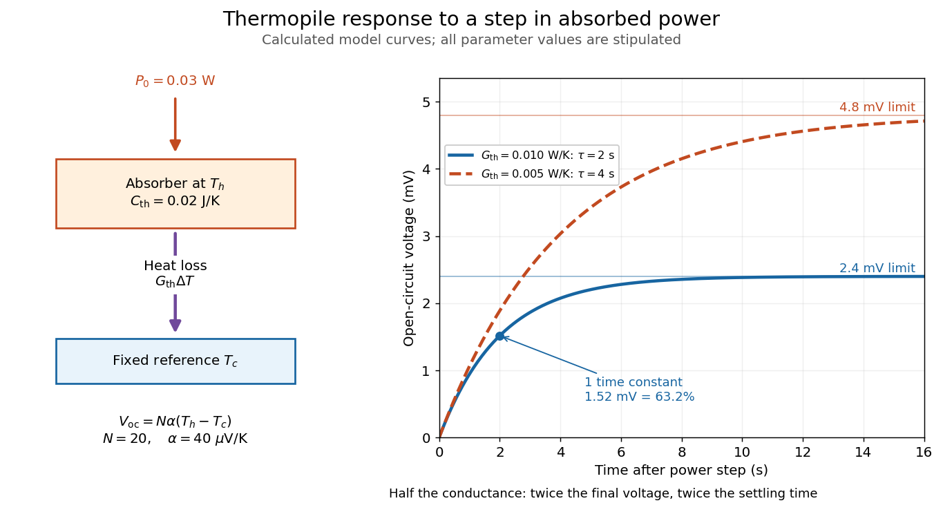
The steady ratio $V_{\infty }/P_0=N\alpha /G_{\mathrm{th}}$ is $0.080\mathrm{V}{\mathrm{W}}^{-1}$ in this constructed model. Halving thermal conductance doubles this ratio but also doubles the time constant if heat capacity stays fixed. Reducing heat capacity alone speeds the response without changing its steady value. Increasing $N$ gives a larger signal only at fixed individual temperature differences: adding legs can also change thermal conductance, heat capacity and electrical resistance. The algebra identifies coupled design choices, rather than predicting a particular manufactured detector.

A finite electrical resistance produces Thermal electrical noise. For nearly uniform absolute temperature $T$ and effective measurement signal bandwidth $B$, its root mean square open-circuit voltage isHere $k_{\mathrm{B}}$ is the Boltzmann constant. Thermal electrical noise in the sensing element is an important contribution, and the signal bandwidth enters its voltage variance.^[ref] If identical pairs have fixed electrical resistance $r$ and fixed $\Delta T$, then $R_{\mathrm{pile}}=Nr$: the signal grows as $N$ while this noise grows as $\sqrt{N}$. The resulting signal-to-noise ratio grows only as $\sqrt{N}$ under those assumptions. Reference temperature drift, environmental electromagnetic radiation, and meter noise remain separate limits; reducing signal bandwidth trades fast information for less integrated electrical noise.

A thermopile absorber converts incident electromagnetic radiation into heat near the thermocouple measuring junctions. Electrically separate junctions can share its temperature through thermal contact. The reference support provides a path for heat transfer and a comparison temperature; “cold” denotes this reference role, even if it is warmer than the absorber.

Distinguish incident power from absorbed power. A window, the illuminated area, and the absorption of the coating determine their relation. A detector's measured voltage sensitivity can depend on where a small illuminated spot lies.^[ref] The model in thermopile thermal response takes absorbed power as its input, so an optical calibration is a separate step.

Use the A-positive terminal order of Seebeck effect for each thermocouple. Its thermocouple measuring junction has temperature $T_{h,i}$ and its reference connections have temperature $T_{c,i}$. Define the difference of Seebeck coefficients as ${\alpha }_i(T)=S_{A,i}(T)-S_{B,i}(T)$. Connect the B reference end of one thermocouple to the A reference end of the next at a common local temperature, so the terminal electric potential differences add:The first A reference terminal is the positive meter input; the final B reference terminal is the negative input. Following this connected path and adding the individual Seebeck effect integrals proves the result. Matched meter leads with common endpoint temperatures cancel as in an isothermal terminal block. The manufacturer's sum formula also allows unequal individual contributions.^[ref]

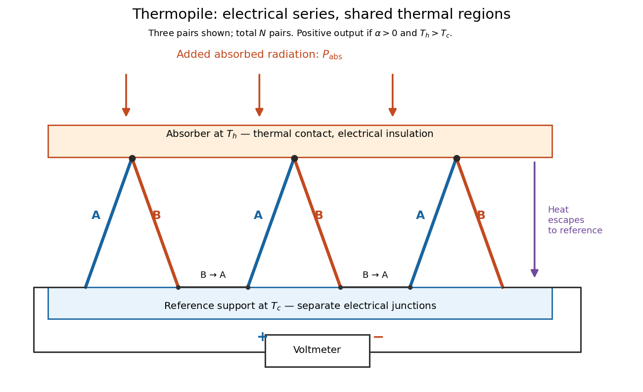
If all pairs share $T_h,T_c$ and the same nearly constant difference $\alpha$ of Seebeck coefficients throughout that temperature interval, thenThis $\alpha$ is the pair's relative Seebeck coefficient, not either material's individual coefficient or a universal device constant. As an original constructed example, choose $N=20$, $\alpha =40\mu \mathrm{V}{\mathrm{K}}^{-1}$ and $\Delta T=5\mathrm{K}$. Each thermocouple contributes $0.20\mathrm{mV}$ andReversing the meter connections changes the sign. Exchanging $T_h$ and $T_c$ reverses the integrals and hence the electromotive force; this reversible sign response does not make a detector with heat conduction a reversible thermodynamic process. Reversing the wiring of one pair instead gives $(N-2)\alpha \Delta T$, because one contribution is subtracted rather than added. For this example the result is $3.6\mathrm{mV}$, and at equal junction temperatures every contribution vanishes.

The open-circuit condition matters. If the array's total electrical resistance is $R_{\mathrm{pile}}$ and the meter input has electrical resistance $R_m$, the elementary voltage divider model gives $V_m=V_{\mathrm{oc}}{R}_m/(R_m+R_{\mathrm{pile}})$. Thus $R_m\gg R_{\mathrm{pile}}$ is needed to suppress voltmeter loading. Appreciable electric current also permits Joule heating and the thermoelectric heat transfer to disturb the assumed junction temperatures.

For a mechanical coordinate $x$ at fixed temperature, total volume and particle numbers, the relevant thermodynamic potential is the Helmholtz free energy $F(x)$. Its generalized force is $f=-F^{\prime }(x)$. At mechanical equilibrium, $f(x_{\ast })=0$, and a linearly restoring force has $f^{\prime }(x_{\ast })<0$, equivalently $F^{\prime \prime }(x_{\ast })>0$. A Taylor expansion then proves a strict local free-energy minimum. If $F$ is a strictly convex function throughout the accessible domain, the stationary state is the unique global minimum.

Thermal conductance is the heat transfer rate divided by the driving temperature difference in a linear contact model. It is the reciprocal of thermal resistance, with units $\mathrm{W}{\mathrm{K}}^{-1}$; thus $\dot{Q}=G(T_1-T_2)$ for heat transferred from body 1 to body 2.

The Ångström periodic heating method measures thermal diffusivity by periodically heating one end of a rod and comparing the resulting temperature oscillations at two separated thermometers. The farther signal has a smaller amplitude and a later wave phase. Their combination measures how quickly the material redistributes heat, without requiring the absolute heater power. The method bears the name of Anders Jonas Ångström, the physicist who became a professor at Uppsala in 1858.^[ref]

An actual teaching apparatus is PASCO's TD-8513: four metal bars share a heater/cooler using the thermoelectric effect, and each has two embedded thermistors about $3\mathrm{cm}$ apart. Foam covers reduce environmental heat transfer. Its manual instructs students to measure sensor spacing and connect the thermistors through a temperature interface to a computer. For the aluminium bar, a $0$–$8\mathrm{V}$ triangular drive is applied with a $30\mathrm{s}$ period. Recording begins after the amplitudes stabilize; two cycles provide amplitudes and the delay between corresponding peaks. Repeated runs at $40$ and $50\mathrm{s}$ test consistency. The manual converts the inferred thermal diffusivity to thermal conductivity using mass density and specific heat capacity.^[ref]

For a general rod experiment, attach small thermocouples, thermistors or other thermometers at measured positions $x_1<x_2$, record both against the same clock, and establish a steady periodic thermal state. A sinusoid is especially convenient. For a switched or triangular drive, isolate the same Fourier series component at both sensors: unrelated peaks in distorted waveforms need not measure that component's phase difference. Subtract each sensor's mean temperature; a steady spatial background does not belong in the oscillating amplitude ratio. Small excursions help keep thermal conductivity, mass density and specific heat capacity constant.

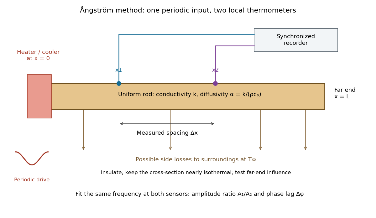
The appeal is that the rod supplies two complementary clocks: decreasing amplitude measures spatial damping, while increasing wave phase lag measures delay. Unlike laser flash analysis, which follows a transient after one pulse, this method repeatedly samples a steady periodic thermal state. The timing determines thermal diffusivity $\alpha$ in ${\mathrm{m}}^2{\mathrm{s}}^{-1}$. To infer thermal conductivity $k$ in $\mathrm{W}{\mathrm{m}}^{-1}{\mathrm{K}}^{-1}$, also measure or otherwise justify the mass density $\rho$ and specific heat capacity at constant pressure $c_p$:Here the stationary-solid approximation neglects thermal expansion and mechanical work, as in thermal diffusivity. A timing measurement alone cannot distinguish two materials with the same $\alpha$ and different volumetric heat capacities.

The translational concentration scale for a nonrelativistic particle in three dimensions, per internal state. It is the inverse cube of the thermal de Broglie wavelength. A classical component with number density $n$ and external one-particle energy $U$ has chemical potential $\mu =k_{B}T\ln (n/n_Q)+U$. An additional internal degeneracy must be included explicitly; it is not hidden in this definition. The dilute classical condition is $n/n_Q\ll 1$ for each occupied internal component.

Kapitza resistance is the thermal boundary resistance encountered between a solid and helium in cryogenics. A cold helium heat bath can coexist with a warmer immersed component under continuous heating. The bath's temperature alone therefore does not establish the component's temperature. Kapitza thermal boundary experiment supplied an early direct demonstration of the obstacle at the solid–liquid boundary.

A microscopic route to interfacial heat transfer is transmission of phonons. Transmission depends on the two materials and their interface; scattering and the condition of the surface matter. ^[ref] The fourth-power thermal boundary model isolates one useful low-temperature limiting law without assigning an empirical coefficient to a particular sample.

Linearity and reversibility answer different questions. The proportional limit ends the interval in which axial stress is proportional to axial strain. Elastic deformation means that deformation is recovered after unloading; a nonlinear response can still be elastic. Conversely, a short straight portion of a loading curve does not by itself demonstrate recovery.

To check recovery, unload and examine the local extensometer strain relative to its initial value, allowing for instrument resolution, drift and any time dependence. A residual extension can indicate plasticity in continuum mechanics, but grip slip can produce a residual in crosshead displacement without the same local residual. Compare the channels before assigning the effect to the specimen. Yield point concerns the onset of irreversible deformation; a specified offset proof stress is an operational convention rather than Young's modulus. For example, a $0.2\%$ offset proof stress is the intersection of the loading curve with $\sigma =E(\epsilon -0.002)$, using the correctly referenced strain. Report the fitted stress/strain window and the unloading evidence alongside the modulus, so that apparatus seating, departure from linearity and onset of plasticity in continuum mechanics remain distinguishable.

Machine compliance is the extra load-path displacement per applied force attributed to the apparatus in a specified measurement model. Its units are $\mathrm{m}{\mathrm{N}}^{-1}$, the reciprocal units of a spring constant. Here $C_m$ includes the frame, load cell, adapters and grips insofar as their deformation contributes to the recorded crosshead displacement $x$. It is a property of that configuration and readout, rather than a universal constant of the testing machine.

Assume a uniform specimen with initial length $L$, constant $A_0$ and Young's modulus $E$, small axial elastic deformation, quasistatic loading, no slip, and a linear, length-independent apparatus response over the chosen force window. Equilibrium makes the same force act through specimen and apparatus, while their extensions add. The two springs in series therefore giveThe offset $x_0$ describes the displacement origin after seating; the slope $q$ describes total compliance. Fitting an intercept avoids forcing an arbitrary zero through the origin, but cannot repair slip or a curved response.

If all of $x-x_0$ is incorrectly attributed to specimen extension, the inferred modulus isFor positive $C_m$, this is too small. The fractional bias is most serious for a short, thick, stiff specimen because its own compliance $L/(E{A}_0)$ is small. A local extensometer instead has $d(\Delta L_g)/dF=L_g/(E{A}_0)$ in this ideal model, excluding deformation outside its contacts.

A shaped specimen requires more care. With varying initial cross-sectional area $A(s)$ and uniform $E$, its axial compliance is $\int ds/[EA(s)]$ in the one-dimensional approximation. Shoulder and end deformation must be included explicitly or remain identical between tests and be absorbed into an effective intercept. Changing only the extensometer gauge length on an unchanged specimen does not change its total compliance and cannot perform a two-length machine compliance separation.

Split one stationary scalar optical field into equal copies travelling at right angles with common transverse linear polarization. For wavevectors $k(\hat{\mathbf{x}}\pm \hat{\mathbf{y}})/\sqrt{2}$, the relative geometric delay is $\sqrt{2}y/c$ in vacuum, while the delay on the $x$ bisector is zero. The electric-field intensity convention gives the displayed pattern and $I(x)=2I_0$. The mean Poynting vector points along $+x$, with magnitude $I(y)/\sqrt{2}$ in that convention. A transverse detector can record the $y$ profile if it resolves the period $\lambda /\sqrt{2}$; a longitudinal $x$ profile is not a transverse camera image.

Two equally intense monochromatic spectral components have normalized first-order optical coherenceThe visibility zeros occur at $\tau =(2j+1)\pi /|\Delta \omega |$, while its revivals repeat every $2\pi /|\Delta \omega |=1/|\Delta \nu |$. This envelope describes self-interference of each spectral component after a delay, not a time-resolved measurement of inter-frequency beating at one fixed point. Unequal line intensities prevent complete cancellation at the minima.

Two delayed copies of the same laser field probe its first-order optical coherence. With equal detected intensities and matched polarizations, the interferometric visibility is $V=|g^{(1)}(\tau )|$. A Lorentzian line shape of frequency full width at half maximum $\Delta \nu$ gives $V=e^{-\pi \Delta \nu |\tau |}$. For a fibre length difference $\Delta l$, the delay is $\tau =n_g\Delta l/c$, where $n_g$ is the group index. Hence $\Delta \nu =-\log V/(\pi |\tau |)$. Replacing $n_g$ by the effective phase index requires negligible dispersion. Polarization mismatch, unequal intensities and uncontrolled phase drift can reduce visibility independently of linewidth.

Counterrotating electron and Positron beams at SPEAR collided inside the Mark I magnetic particle detector. Lead–scintillator scintillation counters identified electrons through large shower pulses; small pulses plus hits beyond the iron return identified muons.^[ref]

The selection required opposite-charge electron–muon tracks, no detected photons, momenta above $0.65\mathrm{GeV}/c$, and transverse noncoplanarity above $20^{\circ }$. Multitrack hadron samples calibrated momentum-dependent misidentification; collinear lepton pairs checked identification losses. Photon and charge control samples tested backgrounds. Acceptance corrections depended on the proposed signal.^[ref]

The 1975 claim was anomalous events without a conventional explanation; new-particle pair production was a possible interpretation.^[ref] Martin Lewis Perl's lecture describes subsequent evidence for a charged lepton.^[ref]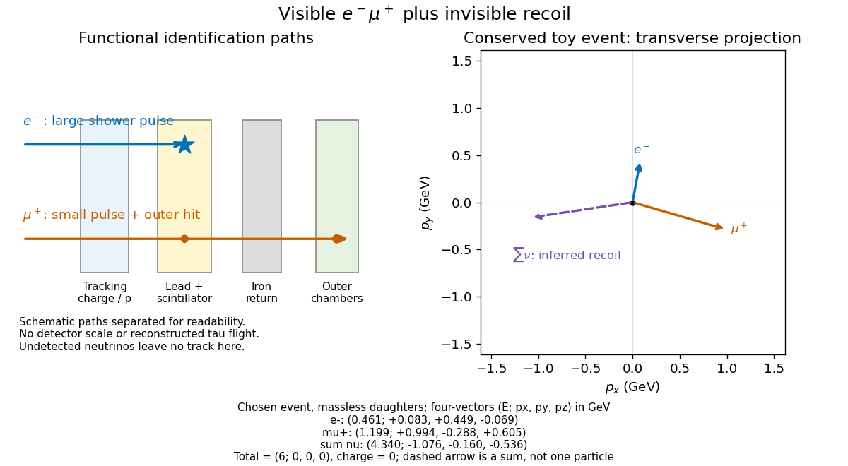

The particle identification problem matters as much as the apparent missing four-momentum in electron-positron collisions. A penetrating hadron can imitate a muon; a particle shower can imitate an electron; an undetected photon or a detector gap can imitate invisible recoil. An absence of additional recorded signals is conditional on detection efficiency. In a proposed signal model, the selected count has the schematic formwhere $\mathcal{L}$ is integrated collider luminosity, $\sigma$ a cross section, and $\epsilon$ the combined acceptance and detection efficiency. A single count cannot determine all three factors. A control sample must probe the relevant momentum and angular range; its abundant events do not automatically calibrate a differently distributed signal.

At a regular point of a differentiable plane curve, the normal line passes through that point perpendicular to its tangent line. If the tangent slope is a finite nonzero number $m$, the normal slope is $-1/m$, since the direction vectors $(1,m)$ and $(1,-1/m)$ have zero dot product. A horizontal tangent has a vertical normal, and a vertical tangent has a horizontal normal. For a regular level set $F(x,y)=c$, the nonzero gradient $\nabla F$ gives a normal direction because differentiating $F$ along the curve gives $\nabla F\cdot {\mathbf{r}}^{\prime }=0$.