
Static Jeans growth-rate spectrum 2026-10-18
Under the Jeans swindle, longitudinal density disturbances in a static uniform gas have . For , one solution grows as with the displayed rate. It decreases monotonically with wavenumber, so the longest available wavelengths grow fastest and the growth-rate supremum is as . There is no preferred finite fastest wavelength in this model. The exact uniform density change is not an ordinary finite-potential Fourier perturbation of the fixed background, and finite-cloud boundaries restrict the available long modes.
Peak frequencies in a standard linear solid Created 2026-10-18 Updated 2026-11-05
For a standard linear solid model with , put . Its storage modulus is and its loss modulus is . The latter peaks at , whereas its loss tangent isDifferentiation puts the loss-tangent peak at , with height . A loss-modulus peak and a loss-tangent peak therefore need not occur at the same frequency. For weak relaxation, is close to one and their frequencies are approximately equal.
Torsion spring Created 2026-10-18 Updated 2026-11-05
An ideal linear torsion spring exerts a restoring torque proportional to the relative angle between its two ends. Integrating the torque gives its elastic potential energy. A spring connecting two rotating bodies contributes to the potential energy; a spring connected to a fixed frame is obtained by setting one angle to zero. The coefficient is the torsional spring constant.
Spinodal decomposition Created 2026-10-18 Updated 2026-11-05
Spinodal decomposition is spontaneous growth of composition fluctuations in a homogeneous mixture whose local mixing free energy has negative composition curvature. For a mean , equal regions at change the mean free energy by , which is negative inside the spinodal. Interfacial costs suppress sufficiently short wavelengths, while conservation of composition constrains the dynamics. Outside the spinodal but inside the binodal, the uniform state is instead metastable and requires nucleation to begin separation.
Magnon Created 2026-10-18 Updated 2026-11-05
A magnon is one quantum of a spin wave, a collective oscillation of magnetic order. Exchange-coupled spins do not fluctuate independently: a disturbance spreads through the ordered system as a mode with a definite wavevector and energy.
In a simple collinear Heisenberg ferromagnet, a single magnon reduces the total spin projection along the ordered axis by one unit of while distributing the disturbance across many sites. At low excitation density, magnon modes can be treated approximately as bosonic oscillators, motivating the Holstein–Primakoff transformation and linear spin-wave approximation. Their population contributes to the reduction of magnetization with increasing temperature. Strong interactions, noncollinear order and large excitation densities can require corrections to the simple independent-magnon picture.
Drift cancellation in a g-factor comparison 2026-10-18
Even a shared field does not cancel if it is sampled at different times. Write and , where . As an original proposed diagnostic, bracket the -state reading at with -state readings at :If , the denominator is exactly , so . A single earlier reading instead gives . For the preceding numerical model and , this unpaired comparison falsely gives approximately ; interpolation recovers . The sequence illustrates cancellation and is not asserted to be Kusch and Foley's exact historical timing protocol.
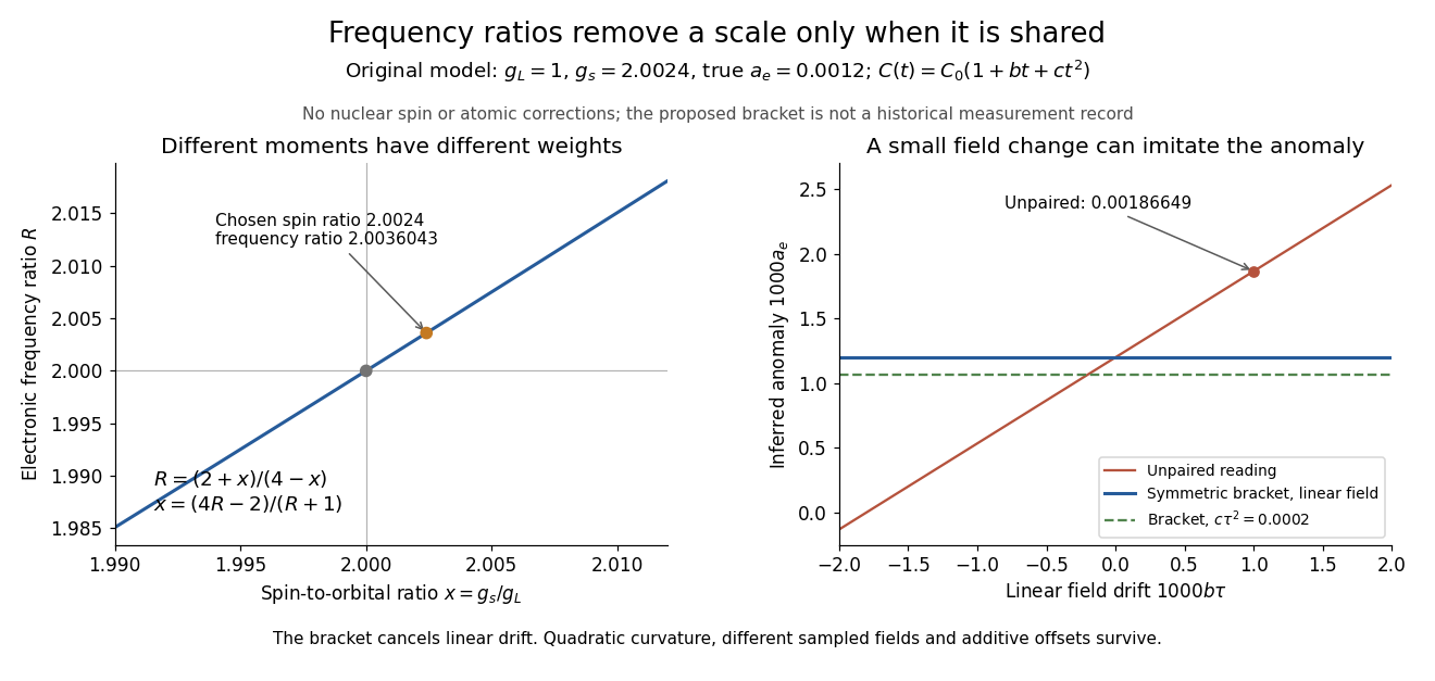
Cancel a shared calibration scale without hiding its limitations
. Original calculations for spin-orbit g-factor ratio from two P states and drift cancellation in a g-factor comparison. All inputs are stipulated. The left plot shows the nonlinear inversion from a frequency ratio to a spin-to-orbital g-factor ratio. The right plot contrasts an unpaired reading with a symmetric bracket under linear field drift; the dashed curve adds chosen quadratic curvature . No curve is a measured resonance or a historical fit. Details.For a curved field , the same calculation givesThe linear drift cancels but the curvature remains. Different fields sampled by the two beams, additive frequency offsets and incorrect atomic corrections also survive. For a small ratio error , direct differentiation of the inverse relation givesRepeated readings can reduce random measurement uncertainty; agreement among genuinely different state comparisons is what tests shared systematic errors in their interpretation.
One-way speed of light 2026-10-18
A one-way speed of light measurement assigns a travel time between spatially separated emission and reception events and therefore requires a distant-clock synchronization convention. In an inertial frame, Einstein synchronisation assigns the vacuum value in either direction. A completed-loop comparison such as the Sagnac effect is a different observable.
Spectrophotometer 2026-10-18
A spectrophotometer measures radiant power in selected wavelength bands. Comparing a chemical solution in a cuvette with a reference blank gives transmittance and absorbance.
Cuvette Created 2026-10-18 Updated 2026-11-05
A sample holder providing a defined geometric light path through a chemical solution for spectrophotometry, as in the trypsin colorimetric assay.
Transverse optical coherence length Created 2026-10-18 Updated 2026-10-20
The transverse optical coherence length summarizes the separation over which equal-time spatial optical coherence remains appreciable. It depends on a contrast criterion and on the source brightness profile. For a distant incoherent source of angular diameter , its characteristic scale is . A uniform circular source gives uniform-disk stellar visibility , with and baseline . Its first zero is . A uniformly bright one-dimensional strip instead has its first zero at ; the numerical factor is a source-model choice, not a universal constant.
Sparse elimination of a four-leaf star 2026-10-18
Take a star graph with center and four leaves . Let be its Laplacian matrix and the identity matrix. In the order , the original example isFor a nonzero vector , its quadratic form isThus is a symmetric positive-definite matrix and either ordering below admits a Cholesky decomposition. Changing the ordering changes the work, rather than the mathematical solvability.
Center first. Eliminating with pivot element leaves the Schur complementEvery pair of leaves now has coupling : six new edges, hence six undirected fill-in positions. The four remaining vertices form a clique. In the Cholesky decomposition, the first column has and . The rest of the lower triangular matrix is dense. To check that later cancellation does not remove its entries, after leaves have also been eliminated, the active leaf block isIndeed a leaf step sends to . All active off-diagonal entries remain negative. The successive pivot elements in ordinary symmetric Gaussian elimination, equivalently the squared diagonals in the Cholesky decomposition, areThe Cholesky decomposition therefore stores nonzero entries, including its diagonal.
Leaves first. Permute to . Each leaf has only one remaining neighbor, so its elimination changes only the center's diagonal, reducing it by . The successive pivot elements are , and the exact Cholesky decomposition isThere is no fill-in, and only nonzero entries in . This is a concrete instance of leaf elimination of a tree-pattern positive-definite matrix; its general proof explains why the same idea works on every tree pattern. The minimum degree algorithm also chooses a leaf at every nontrivial stage of this particular example, but that success gives no general optimality guarantee.
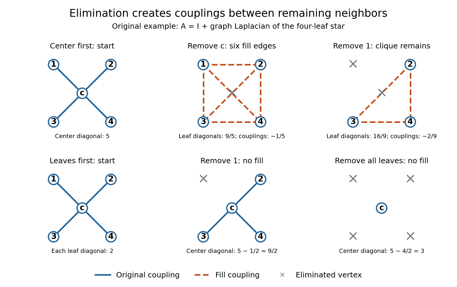
Eliminating the center of a four-leaf star graph creates a clique; eliminating leaves creates no fill-in
. Details. 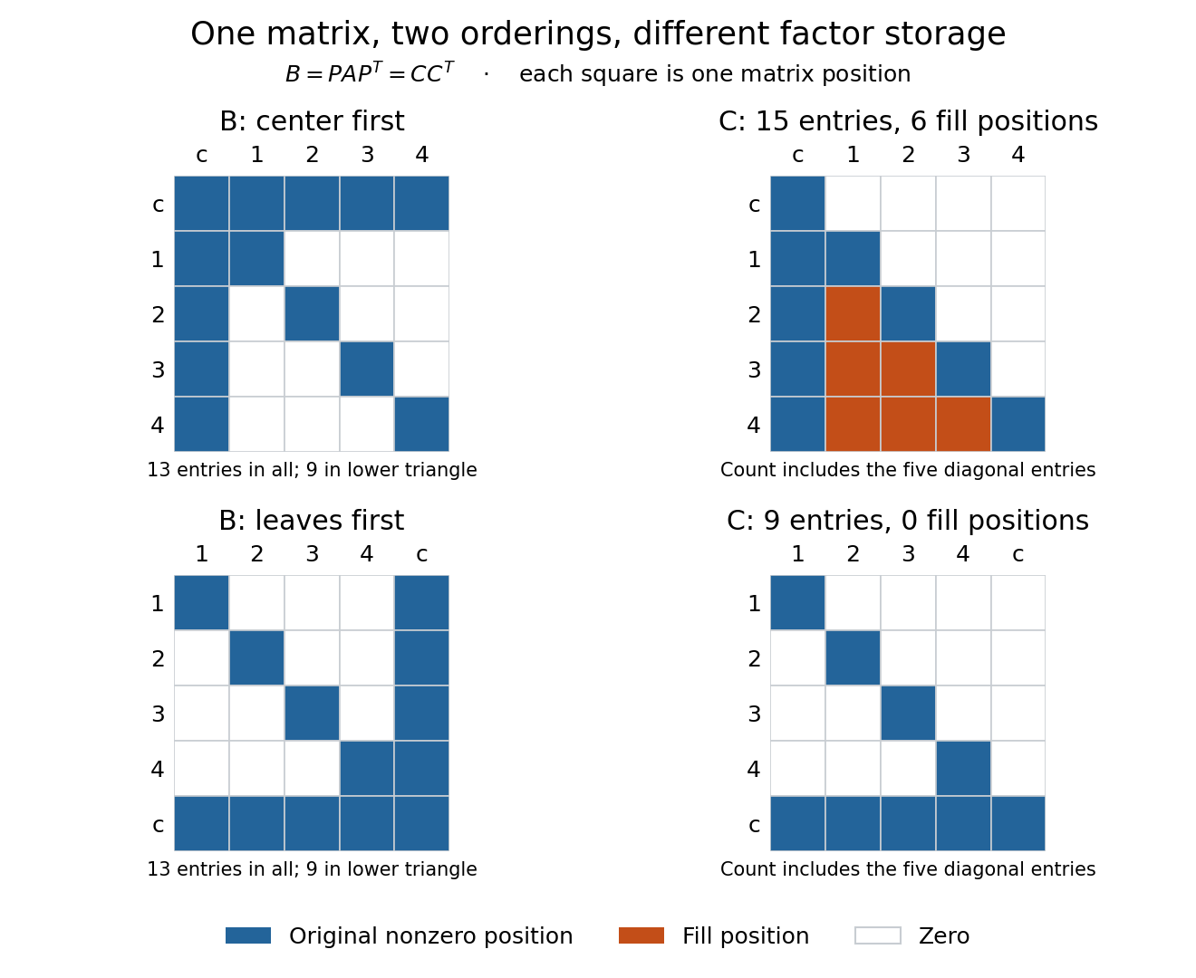
The same symmetric positive-definite matrix has 15 or nine nonzero Cholesky decomposition factor entries, depending on its ordering
. Details. The input has 13 nonzero matrix elements when both symmetric halves are counted, or nine in its lower triangle. The six added undirected edges correspond to six added positions in one triangular factor, or 12 positions if both symmetric halves of the filled pattern are displayed. Comparing all 13 input entries directly with the 15 entries of would mix counting conventions.
Solar neutrino detection Created 2026-10-18 Updated 2026-11-05
Solar neutrino detection asks how an invisible electron neutrino from the Sun becomes a measurable laboratory record. The Homestake experiment stores a reaction product for later counting; Kamiokande records light promptly. The former measures an exposure-integrated rate, whereas the latter can retain event times and statistical source-direction information. These are complementary ways to connect stellar nuclear fusion with neutrino astronomy.
A detector samples a weighted part of a neutrino flux, rather than counting every passing neutrino. For a target population , an ideal reaction rate iswhere is the differential electron neutrino neutrino flux and is the relevant cross section. A detection efficiency belongs inside the integral if it depends on energy. Two detectors can therefore disagree in raw count rate while observing the same source. Interpreting a deficit requires both a source prediction and a detector response.
Solar-cell fill factor 2026-10-18
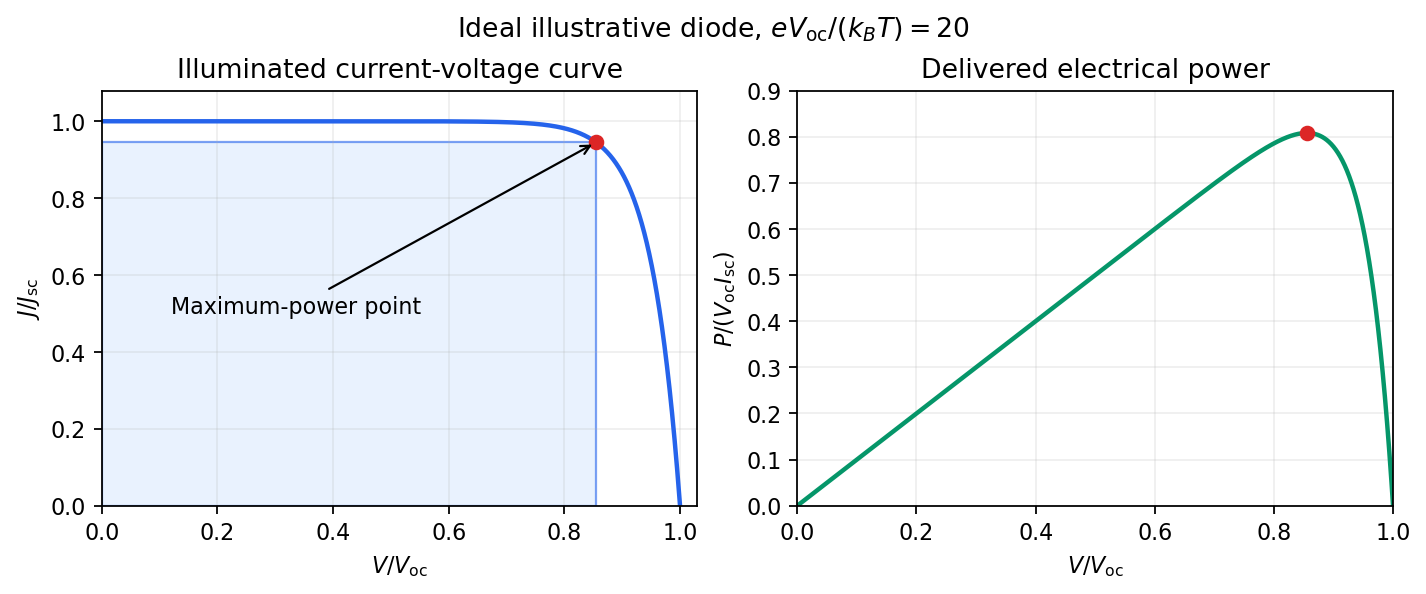
The solar-cell fill factor compares the maximum delivered electrical power with the rectangle formed by the open-circuit electric potential difference and short-circuit electric current. It measures the shape of the illuminated current-voltage characteristic. The conversion efficiency is .
Shockley-Queisser limit Created 2026-10-18 Updated 2026-10-20
The Shockley-Queisser limit is the radiative conversion-efficiency bound for an ideal single-junction solar cell, with one collected electron-electron hole pair per absorbed above-gap photon, carrier thermalization, and radiative recombination required by the reverse optical process. Photons below the band gap are not absorbed, while excess photon energy above it is thermalized. Maximizing the electrical power over the operating electric potential difference and then the band gap gives a ceiling of roughly thirty percent for ordinary unconcentrated sunlight; its precise value depends on the incident spectrum, cell temperature and emission geometry. The original calculation by William Shockley and Hans-Joachim Queisser obtained approximately at for a blackbody source and a cell at .[ref]
Measuring a solar cell's current-voltage characteristic Created 2026-10-18 Updated 2026-10-20
Keep the illumination and cell temperature approximately constant. Connect an ammeter and an adjustable resistor as a series circuit across the solar cell; connect a high-resistance voltmeter across its terminals. Vary the electrical resistance and record pairs of electric potential difference and delivered electric current . This measures the illuminated current-voltage characteristic.
A load close to a short circuit estimates at . With the load disconnected, an open circuit measurement using a high-resistance voltmeter estimates at . Neither endpoint delivers useful power: vanishes there. The intermediate readings locate the maximum of and determine the solar-cell fill factor. Holding illumination fixed matters because the photogenerated electric current changes with light intensity; holding temperature fixed matters because the diode saturation current and junction response change with it.
This experiment distinguishes producing an electric potential difference from delivering energy to a load. To determine conversion efficiency as well, measure the incident power on the illuminated area, rather than equating it to a lamp's electrical rating.


SN 1987A neutrino burst Created 2026-10-18 Updated 2026-10-20
The original Kamiokande paper reported a low-energy event cluster on 23 February 1987 above surrounding background. Inverse beta decay, , provides an electron antineutrino channel through Positron light. Neutrino-electron elastic scattering is more directional. The burst supported core-collapse supernova neutrino emission, with limited statistics and channel ambiguity.[ref]
Observation of a Neutrino Burst from the Supernova SN1987A by K. Hirata and others. pp. 1490–1493; Fig. 2, Table I and discussion
An original counting illustration shows why timing matters. Suppose an independently measured background is a Poisson process of rate . In a prespecified window , the probability of at least two background events isFor the synthetic choice , this is about , obtained by subtracting the zero- and one-event probabilities of the Poisson distribution. The Homestake experiment's delayed extraction cannot supply such capture-time clustering. This calculation is not a significance estimate for SN 1987A: searching many possible windows, varying acceptance and correlated backgrounds change the inference.
Transconductance 2026-10-18
The change of output electric current per change of input electric potential difference, evaluated at an operating point with the other terminal conditions specified. In a small-signal model, describes this contribution; transconductance has the dimensions of electrical conductance.
Counterbalanced gyroscope precession 2026-10-18
Let a horizontal gyroscope have signed spin angular momentum along the axle. The disk's centre of mass is at and a counterweight is at . Gravity supplies torque . Since , steady horizontal precession gives the displayed signed vertical angular velocity. Neglect the axle's mass and the counterweight's axial spin moment of inertia. The zero-torque choice allows the axle to remain fixed. Moving the counterweight through this position reverses the gravitational torque and the associated slow precession.
Neutron moderation 2026-10-18
Neutron moderation reduces the kinetic energy of fast neutrons through repeated collisions in a neutron moderator. In a simple elastic collision model, hydrogen is especially effective because a proton and a neutron have nearly equal masses: the maximum elastic recoil energy fraction can approach one. The mean logarithmic energy decrement describes typical accumulated slowing, whereas the maximum transfer describes a single endpoint.
Slowing, absorption and escape compete. A material can remove neutrons by neutron capture before they become thermal neutrons, and some neutrons escape its boundaries. Describing a neutron moderator therefore requires more than collision kinematics. Near thermal equilibrium, target thermal motion can also give energy back to a neutron; the initially stationary target approximation must then be replaced.
Thermal neutron 2026-10-18
A thermal neutron belongs to a population approximately in thermal equilibrium with its surroundings. Such a population has a distribution of kinetic energies, not one fixed energy. The scale uses the Boltzmann constant and thermodynamic temperature; it is about at . The mean translational kinetic energy for a classical three-dimensional equilibrium population is . Not every slow neutron has reached this equilibrium.
There are unlisted articles, also show them or only show them.