
Fluorescent screen Created 2026-10-18 Updated 2026-10-20
A screen whose fluorescence makes the spatial distribution of incident electrons or other radiation visible.
Quenching (fluorescence) Created 2026-10-18 Updated 2026-10-20
A reduction in fluorescence caused by a process competing with photon emission, for example a collision that removes excitation energy without emitting a photon. Measuring less light because fewer excitation photons reach the sample does not by itself establish fluorescence quenching.
For composition-independent , the spinodal of Flory–Huggins solution theory is . At its thermodynamic critical point, a second condition gives , proving the displayed values. Hence and . Under , the theta temperature is and . Thus approaches a constant while scales as . Converting to a temperature always requires a specified or inferred law.
Flory interaction parameter 2026-10-18
The Flory interaction parameter measures the excess free-energy cost of unlike contacts in Flory–Huggins solution theory. For a simple lattice of coordination number and contact energies , and ,Real effective parameters may also contain entropic contributions and composition dependence. With site volume and composition-independent , the effective two-segment excluded volume is . Positive, zero and negative correspond respectively to a good solvent, the theta temperature condition and a poor solvent. In particular, means cancellation of leading repulsive and attractive contributions; it does not mean that every molecular interaction vanishes.
Osmotic pressure in Flory-Huggins solution theory Created 2026-10-18 Updated 2026-10-20
Let be the mixing free energy per lattice site in Flory–Huggins solution theory, the site volume, and the polymer volume fraction. The solvent mixing chemical potential is , so its balance against the pure-solvent pressure contribution gives . For composition-independent ,The first term is the ideal chain translational contribution; the second encodes the effective two-segment excluded volume. At the theta temperature condition it vanishes but the positive third-order term remains. Treating as a free-energy density without dividing by loses the physical dimensions of osmotic pressure.
Carrier density from spin-degenerate quantum oscillations Created 2026-10-18 Updated 2026-11-05
One resolved spin branch of a two-dimensional Landau level has degeneracy per area. Thus the total carrier density is , where the filling factor counts all occupied spin and other internal branches, including partial filling. If consecutive unsplit orbital peaks change filling by an unresolved degeneracy ,For only spin degeneracy, . Once spin splitting is resolved, adjacent individual branches differ by one rather than two; counting split subpeaks as unsplit orbital peaks gives a factor-two error.
Loop Feynman diagram 2026-10-18
A connected loop Feynman diagram has at least one independent internal loop momentum. With internal lines and vertices, the number of independent loops is . A tree-level Feynman diagram has . A multi-leg amplitude generated by a loop is not an extra fundamental interaction vertex of the original Lagrangian.
Feynman rules Created 2026-10-18 Updated 2026-11-05
Feynman rules translate a Feynman diagram into a contribution to a scattering amplitude or correlation function in perturbation theory. They specify factors for external states, interaction vertices, internal propagators, momentum-conservation constraints and loop integrals, with statistics-dependent signs and symmetry factors. For quantum electrodynamics, a photon-fermion vertex contains the coupling , while a photon propagator supplies an inverse squared four-momentum. The complete amplitude also contains currents, so propagator powers alone do not determine the energy dependence of a scattering cross-section.
Magnetic compensation temperature 2026-10-18
At a magnetic compensation temperature, : an ordered ferrimagnet has zero net magnetization. Such cancellation need not occur in every material.[ref]
Magnetism and the local molecular field by Louis Néel. §8, Fig.7; §§11–12, pp.335–338: cancellation within an ordered phase
For an original stipulated example, let , with , and prescribe sublattice magnitudes per common volume byTake A along and B along , retaining a fixed sublattice orientation convention. These are toy functions, not measured curves or a self-consistent mean-field approximation. Their difference factors exactly:At , . At , both magnitudes equal and : this is compensation with finite order. At , . At , both magnitudes vanish: that endpoint represents the stipulated Curie temperature, not another compensation point. For stipulate both ordered magnitudes zero; do not extrapolate the polynomials into negative sublattice magnitudes.
The sign change refers to the net component relative to the fixed A direction. A freely reorienting specimen in an applied magnetic field need not display this signed branch directly. The example isolates the cancellation mechanism; it predicts neither a material's transition temperature nor its response to magnetic domains or an applied magnetic field.
Fermi contour 2026-10-18
For a two-dimensional energy band, a Fermi contour is the set of wavevectors at the Fermi energy. It is the two-dimensional counterpart of a Fermi surface. At a regular value it consists locally of curves; at a band extremum or a crossing it can acquire isolated points or intersecting branches. At zero temperature, each band's occupied region satisfies , so the contours must be labelled by band when determining occupations. The Fermi contours of an isotropic Rashba band illustrate why two contours need not belong to two different bands.
Fermi point Created 2026-10-18 Updated 2026-11-05
A Fermi point is a point of the zero-temperature Fermi surface in one-dimensional momentum space. For a spin-degenerate band with one occupied interval, its two boundaries are usually and . Low-energy excitations near them form left- and right-moving branches. A perturbation at wavevector can mix those branches, as in a Peierls distortion.
Sommerfeld expansion Created 2026-10-18 Updated 2026-10-20
The Sommerfeld expansion approximates integrals weighted by the Fermi-Dirac distribution when and is smooth near . Applying it to the number integral at fixed particle number gives . The sign depends on the slope of the density of states. For an unbounded parabolic band, , yielding opposite quadratic shifts in one and three dimensions. In two dimensions the leading algebraic shift vanishes, but the finite band-bottom cutoff still gives an exponentially small negative shift.
Pickup coil Created 2026-10-18 Updated 2026-11-05
A pickup coil converts changing magnetic flux into an electromotive force through Faraday's law of induction. For identical turns linking flux per turn, the ideal open-circuit signal is .
Move a magnet toward the coil, stop it and withdraw it: approach and withdrawal give opposite signal signs, while a stationary magnet gives no ideal induction signal despite its nonzero magnetic field. This makes the coil a change detector rather than a direct static-field meter. Coil area, orientation, winding resistance and readout loading determine the actual voltage and noise; integrating a calibrated signal can infer a change of flux.
Faraday induction-ring experiment 2026-10-18
Michael Faraday's induction ring separates two questions: can one electrical circuit affect another without an electrical connection, and does that effect continue under steady conditions? The surviving apparatus uses insulated copper windings around an iron ring; the Royal Institution dates the successful experiment to 29 August 1831.[ref]
Michael Faraday's ring-coil apparatus by Royal Institution. Collection record, date, materials and Description
Faraday connected one winding group to a battery, the other to a galvanometer. Making battery contact deflected the needle; maintaining contact let it return to rest; breaking contact reversed the response. Reversing the battery reversed the deflections. His separate cylinder comparison enhanced induction with iron, whereas replacing it with copper gave no enhancement over the windings alone.[ref]
Experimental Researches in Electricity, Volume 1 by Michael Faraday. First Series, §§27–30, ring, connections and reversal; §§34–35, distinct cylinder comparison
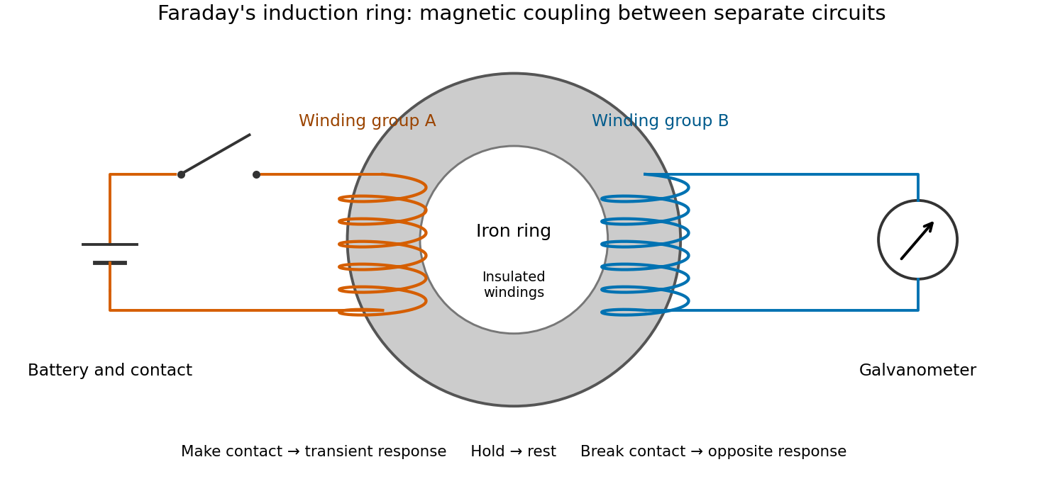

The contrast between a switching response and a quiet steady state makes mutual induction tangible. A steady primary electric current can maintain magnetic flux without sustaining a secondary electromotive force. Changes in magnetic flux linkage matter, as expressed by Faraday's law of induction. This is why a driven electrical transformer uses repeated changes in magnetic flux to supply secondary power.
The galvanometer readout of an induction pulse also separates the measured motion from the inferred electric current. Its moment of inertia and damping mean that a deflection is not an instantaneous trace of electric current. The following coupled RL induction model calculates currents in a stipulated circuit, rather than fitting Faraday's needle motion or reconstructing his switching times.
Induced current in a tilted resistive loop 2026-10-18
Choose the positive loop normal and its positive circulation by the right-hand rule. A spatially uniform external magnetic field of fixed direction and signed magnitude , at angle to that normal, gives magnetic flux . Neglecting the loop's self-inductance, Faraday's law of induction and Ohm's law give the displayed electric current. At a quarter-cycle the external field is zero but its normal component is decreasing most rapidly, so the current produces a field in the direction of the initial normal flux, as required by Lenz's law. With appreciable self-inductance the circuit instead obeys .
Uniform gravity-driven Newtonian film Created 2026-10-18 Updated 2026-11-05
A uniform steady film of thickness on a plane inclined by above horizontal has downslope coordinate and outward normal coordinate . Neglecting air shear, the pressure is and its downslope gradient vanishes. The Newtonian fluid momentum equation is . The no-slip boundary condition and shear-free free surface give the displayed parabolic profile. Integrating over thickness gives volume flux per unit width . The wall shear balances the film's downslope weight, and the vertical-wall case is .
Difference of two cubes 2026-10-18
The polynomial identityfollows by multiplying out the right side. For real , the quadratic factor is , so it is nonnegative and vanishes only when . The identity is a special case of the finite geometric series factorisation .
Sum of two cubes Created 2026-10-18 Updated 2026-10-20
Replacing by in the difference of two cubes givesFor real cube roots and , this simplifies to . Specifying real cube roots matters when using such identities with negative real inputs; unconstrained complex exponentiation has logarithm-branch choices.
Extreme point that is not an exposed point 2026-10-18
The distinction appears at a smooth join between a straight segment and a curved boundary. Consider the convex hullThe upper tangent from meets the unit circle at . The supporting line isEvery point of the unit disk has , with equality only at . Hence the convex face of where equality holds is exactly the line segment .
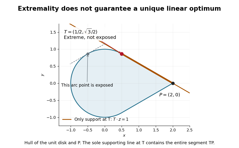
An extreme point can fail to be an exposed point
. Original analytic convex hull of the unit disk and . The tangent contact is extreme, but its only supporting line contains the entire line segment . A different marked point on the curved arc is exposed by its own tangent line. Details.
The point is extreme. If a nontrivial convex combination of two points of equals , both must belong to the convex face . Since is an endpoint of that line segment, both must equal .
Yet is not exposed. A nonzero linear functional maximizing at on must also maximize there on the included unit disk. Its vector must be a positive multiple of , by the equality condition in the Cauchy-Schwarz inequality. It then gives the same value as . No linear functional can select alone. Being an extreme point is a property of possible mixtures; being an exposed point adds the ability to distinguish it by one linear objective.
Exposed point 2026-10-18
An exposed point is a point uniquely selected by maximizing a linear functional. In , a point of a convex set is exposed if some vector satisfiesGeometrically, a supporting hyperplane touches the convex set only at . Every exposed point is an extreme point: a convex combination that attains the maximum can put positive weight only on maximizers, and there is only one.[ref]
Convex geometry (BME course BMETE94AM22). §6, Definition 6.2 and Proposition 6.7, printed pp. 36–37: exposed points and their inclusion among extremal points
The unit disk calculation in extreme point exposes every point of the unit circle. For a corner of the square, exposes it: attains two only at . However, maximizing exposes no single point on the right edge, since all of them have the same objective value. A linear functional may have several optimal points, even when some of them are extreme.
There are unlisted articles, also show them or only show them.