
Holographic object wave 2026-10-18
A holographic object wave is the object-dependent field arriving at the recording surface, including the propagation from the object. Its complex amplitude generally differs from the transmission function at the object itself. Distinguishing these two planes is essential when refocusing a hologram.
Holographic reference wave 2026-10-18
A holographic reference wave is a known coherent comparison field at the recording surface. Its wave phase supplies the standard against which the holographic object wave is encoded. In in-line holography, the undiffracted part of the illumination can supply this field; in off-axis holography, a separate tilted beam supplies it.
Hologram 2026-10-18
A hologram is the recorded wave interference pattern used for holographic wavefront reconstruction. The pattern need not resemble the object. A photographic emulsion stores a material change produced by exposure; a digital intensity record instead requires numerical reconstruction or a device that displays the corresponding optical modulation.
Electron holography Created 2026-10-18 Updated 2026-10-20
Electron holography uses electron object and reference waves to encode their relative wave phase in a hologram.[ref]
Work by Hiroyuki Noji Created 2026-10-18 Updated 2026-10-31
Four-terminal sensing tests a conducting connection between the voltage contacts. A magnetometer instead tests the sample's magnetic response. These measurements provide complementary constraints: the first is sensitive to a continuous path, while the second also depends on screening geometry and preparation history.
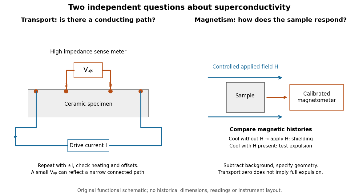

For transport, define between the inner contacts and use the reversed-electric current estimator from four-terminal sensing. Contact separation excludes drive-contact drops, but does not eliminate a drifting thermoelectric effect, Joule heating or an unrepresentative path through part of the specimen. Repeat at smaller electric currents and compare results at the same sample temperature. A finite-current result refers to that electric current and its relation to the path's superconducting critical current.
For magnetism, distinguish cooling in zero applied magnetic field and then applying it from the Field-cooled Meissner experiment. Record the applied magnetic field, background and sample geometry when interpreting magnetization or magnetic susceptibility. A transport short does not establish full Meissner effect screening throughout the specimen. Conversely, flux pinning in a type-II superconductor can make the field-cooled magnetic response differ from ideal complete expulsion. Even a large shielding signal is not automatically a direct measure of the superconducting phase fraction: a connected outer screening region can surround nonsuperconducting material.
Bednorz-Müller experiment 2026-10-18
In 1986, Johannes Georg Bednorz and Karl Alexander Müller precipitated mixed oxalates from aqueous barium, lanthanum and copper nitrates using oxalic acid. Heating at for five hours preceded pressing at and reheating for sintering. X-ray diffraction resolved three phases. Rectangular pieces carried gold electrodes and indium wires; four-terminal sensing in a continuous-flow cryostat measured electrical resistance versus temperature. Annealing atmosphere and measuring electric current density were varied; larger electric current densities suppressed the drop. An onset near differed from the much lower temperature where the drop approached three orders of magnitude.[ref]
This was evidence for possible granular superconductivity, with phase identification unfinished. The paper deferred Meissner effect and heat capacity tests; its proof note corrected bulk lanthanum/barium ratios. A resistive onset did not establish a uniform bulk superconducting transition temperature.[ref]
Possible high Tc superconductivity in the Ba-La-Cu-O system by Johannes Georg Bednorz and Karl Alexander Müller. §IV, p.192; proof note, p.193
Their 1987 authored lecture describes later magnetometer checks on lead, followed by magnetic susceptibility measurements: samples with a resistive drop developed diamagnetism at somewhat lower temperatures. Combining magnetic, transport and X-ray diffraction results identified barium-substituted as the superconducting phase. These later results strengthened the case beyond the initial mixed-phase transport evidence.[ref]
Cuprate superconductor Created 2026-10-18 Updated 2026-11-05
A cuprate superconductor is a copper-oxide material exhibiting superconductivity, with layered copper-oxygen units central to its crystal structure. Chemical composition and oxygen content must accompany a quoted superconducting transition temperature; the nominal recipe of a mixed-phase pellet is not the composition of its superconducting constituent. The formal hole count in a cuprate illustrates the distinction between composition and electronic interpretation.
The University of Washington's Decomposition of H₂O₂ with MnO₂ describes a supervised demonstration using solid manganese dioxide and hydrogen peroxide listed as 30%. Its cylinder version uses a spatula to introduce the solid; the stated readout is immediate molecular oxygen bubbles and heat production. An alternate bottle version replaces the contents of a tea bag with the solid and suspends it above the liquid. Releasing the bag brings it into contact with the liquid. The bag-above-liquid stage supplies a before-contact comparison; the page gives no timed gas collection, replicated blank trials or quantitative reaction rates.[ref]
Decomposition of H₂O₂ with MnO₂ by University of Washington Department of Chemistry. Chemicals and Solutions; Materials; Procedure; Alternate Procedure: Genie in a bottle, apparatus and steps 3–6
The balanced net chemical equation is . Appearance of gas after contact supports a contact-dependent acceleration of decomposition under these conditions. It does not distinguish surface conversion from a contribution of dissolved material, establish regeneration, or measure an activation energy. The simultaneous heat release also means that temperature can change after contact. A matched no-solid comparison and an empty-bag comparison would test background decomposition and the bag's contribution; these are proposed controls, not reported trials. The catalysed peroxide comparison supplies a complementary inspected teaching experiment with separate single-addition and paired-addition comparisons.
Catalyst particle size and accessible area 2026-10-18
Consider an original geometric model of separate nonporous solid spheres, each with radius . Hold their total volume fixed. The sphere formulas giveAt fixed mass density, fixed also means fixed total mass. Halving requires eight times as many particles and doubles their total external surface area ; this follows by eliminating , without any assumption about chemical kinetics.
For example, take one sphere of radius , so . Eight spheres of radius have the same . Their total surface areas are respectively and , approximately and . Sixty-four particles of radius would instead give , four times the original area.
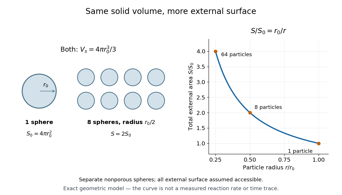

To obtain a kinetic prediction, add assumptions explicitly. Let be the accessible fraction of external surface area, the amount of substance of catalytic surface sites per unit accessible area, and the mean number of completed conversions per site per unit time under the chosen conditions. Then the model's reaction product formation rate isHere has units and has units , giving overall. Halving doubles this predicted rate only if , and remain unchanged. Particle contact can hide area; pores can add area; diffusion, altered surface structure and catalyst deactivation can change the other factors. Consequently, twice the calculated external area is not a universal promise of twice the measured reaction rate. The geometric argument changes contact, not the net Gibbs free energy or the equilibrium constant of the same overall chemical reaction.
Catalytic surface site 2026-10-18
A catalytic surface site is a location on a solid surface capable of participating in a catalytic route. The schematic notation denotes a vacant site; denotes A bound there. A minimal illustrative catalytic cycle isThe first step represents adsorption; the second combines conversion and release. Cancelling and gives . The site is regenerated even though its occupancy changes during the cycle. This is an original bookkeeping model, not a measured reaction mechanism for manganese dioxide.
If the only site states are vacant and occupied by A, the site inventory obeys . A blocked or inaccessible part of a particle does not contribute available catalytic surface sites merely because it contributes mass. Different surface structures can have different abilities to bind and convert reactants; equal geometric surface area need not mean equal catalytic activity.
Dirichlet and Neumann spectra of a square 2026-10-18
For on the square, separation of variables gives Dirichlet eigenfunctions with , and Neumann eigenfunctions with . The eigenvalues in both cases are , with multiplicity equal to the number of ordered admissible pairs. In particular, an arbitrary expression with integers need not be a Dirichlet eigenvalue when one index is zero. The Neumann zero eigenvalue has the constant eigenfunction, whereas the Dirichlet zero problem has only the zero solution by Dirichlet uniqueness for the Poisson equation.
Radial Dirichlet modes of a spherical cavity 2026-10-18
A bounded spherically symmetric solution of the Helmholtz equation in a ball with zero value at radius satisfies . The substitution gives with , so the displayed modes have ; the apparent singularity at zero is removable. Their Rayleigh quotient is . The trial profile gives the upper bound , compared with the exact lowest value . Boundedness at zero eliminates the solution and makes the endpoint term in the Sturm-Liouville problem vanish.
Zimm-Bragg model Created 2026-10-18 Updated 2026-10-25
A homogeneous Zimm-Bragg chain assigns propagation weight to each helical unit and initiation factor to each helical run. With states ordered as coil and helix, one possible transfer matrix for a classical spin chain isIts largest eigenvalue is . In the long-chain limit the partition function grows as , so logarithmic differentiation gives the helical fraction , equal to the displayed expression. If , thenFor , and units are noncooperative. A small initiation factor suppresses boundaries and sharpens the crossover around , with width of order . For every fixed the long-chain expression is smooth; a discontinuous step appears only in the singular limit. [ref]
https://doi.org/10.1063/1.1730390. Theory of the Phase Transition between Helix and Random Coil in Polypeptide Chains, Journal of Chemical Physics 31 (1959), 526–535: propagation and initiation parameters and characteristic-matrix solution
Transverse nuclear magnetic resonance measures absorption from a radio-frequency magnetic field perpendicular to the static field. In the A phase, the resonance moved above the Larmor frequency; in the B phase it returned to that frequency despite the changed state. Anthony James Leggett connected the shift to collective spin-orbit structure. A predicted longitudinal resonance, driven parallel to the static field, supplied a further B-phase test.[ref]
Nobel Lecture: Superfluid 3He: the early days as seen by a theorist by Anthony James Leggett. pp.1002–1003 and1009, transverse geometry and longitudinal test
The helium-3 superfluid discovery experiment establishes why a new phase was inferred; comparing response channels then tests its internal structure. An unchanged peak in one geometry cannot, by itself, establish that nothing ordered.
Spin-triplet p-wave pairing 2026-10-18
Spin-triplet p-wave pairing has pair spin and orbital angular momentum , allowing multiple order parameters beyond conventional BCS theory with zero orbital angular momentum. [ref]
The Extraordinary Phases of Liquid 3He by David Morris Lee. Lee, 1996 lecture; 1997 reprint p.658
Specifying this symmetry does not determine its microscopic attraction mechanism. A short exchange-symmetry check explains why these quantum numbers fit fermions. The spin-one-half triplet states , and are symmetric under exchange. A stipulated orbital factor proportional to relative momentum changes sign under . Multiplying any symmetric spin function by that odd orbital factor gives an antisymmetric pair wave function, as required by Fermi-Dirac statistics. By comparison, an even s-wave orbital factor needs the antisymmetric spin singlet state. This checks compatibility with exchange statistics; it neither selects a stable phase nor derives its transition temperature.
Pomeranchuk cooling 2026-10-18
Low-temperature solid helium-3 can have greater entropy than the liquid through disordered nuclear spins, enabling compression cooling. [ref]
The Pomeranchuk Effect by Robert Coleman Richardson. Richardson, 1996 lecture, p.91, introduction and Fig.1
The sign follows from the Clapeyron equation. Let be molar entropies and molar volumes of liquid and solid, respectively, on their phase coexistence curve. Equality of their chemical potentials, with , givesWith and , the slope is negative. Reversibly freezing one mole at fixed temperature requires heat into the sample,Here uses the melting convention for latent heat of fusion. This is the opposite sign from ordinary ice melting. The inequalities specify the regime; freezing does not universally cool a substance. In an approximately isolated sample, the growing higher-entropy phase draws on the sample's thermal energy instead of an external heater. Irreversible losses and incoming heat oppose the cooling.
Helium-3 superfluid discovery experiment 2026-10-18
David Morris Lee, Douglas Dean Osheroff and Robert Coleman Richardson compressed coexisting liquid and solid helium-3 in a cell precooled by a dilution refrigerator. Helium-4 pressure drove coupled bellows and a piston; a capacitance diaphragm gauge read pressure and platinum nuclear magnetic resonance supplied thermometry. Uniform compression revealed a slope break A and a small pressure drop B; decompression and varied solid fraction checked reproducibility. Their April 1972 paper, Evidence for a New Phase of Solid He3, interpreted a new solid phase, without establishing liquid superfluidity. [ref]
Evidence for a New Phase of Solid He3 by Douglas Dean Osheroff and others. 1972, pp.885–888, Figs.1–3
The October follow-up replaced the thermometer assembly with a sample nuclear magnetic resonance coil. An applied magnetic field gradient selected different sample layers, separating strong solid signals from the liquid background. At A the liquid resonance shifted; at B its shift disappeared and its magnetic susceptibility fell. Removing the gradient resolved the frequency shift directly. Independence from solid fraction and distinct relaxation times supported the liquid assignment. Thus the reinterpretation rested on phase-selective evidence, rather than relabeling the first paper's title. These magnetic observations identify changed liquid phases; they do not directly measure frictionless flow. [ref]
New Magnetic Phenomena in Liquid He3 below 3 mK by Douglas Dean Osheroff and others. 1972, pp.920–923, Figs.1–3
Douglas Dean Osheroff recalls the subsequent p-wave interpretation. [ref]
Superfluidity in 3He: Discovery and Understanding by Douglas Dean Osheroff. 1996 lecture, p.73
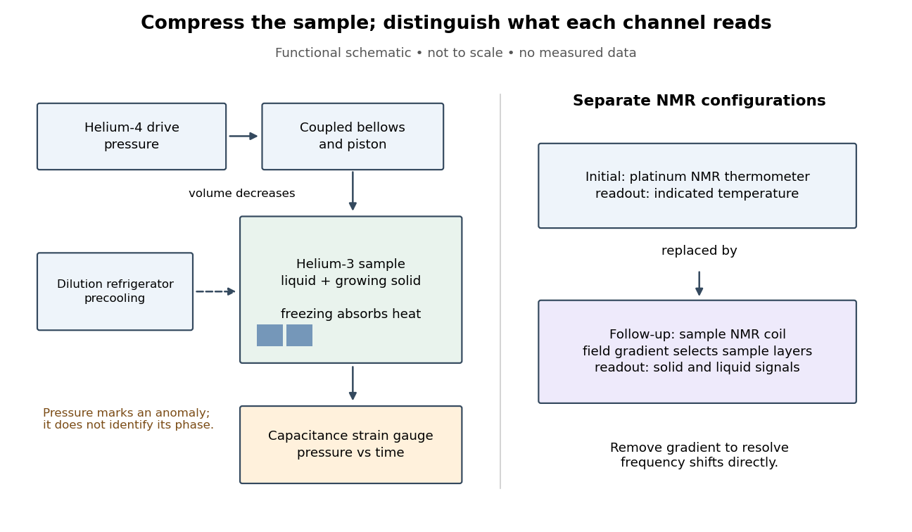
Compression and independent readout channels in the helium-3 superfluid discovery experiment
. Original functional diagram, not a reconstruction to scale. Left: drive, sample and pressure channel. Right: separate thermometer and sample nuclear magnetic resonance configurations; the latter replaces the former in the follow-up. Connections indicate function, not historical wiring. Details.
The inference has a useful limit. A pressure anomaly in two coexisting phases cannot, by itself, identify which phase changed: both contribute to the common phase coexistence curve. Thermometer lag, a temperature gradient or slow equilibration can also separate indicated temperature from the sample state. Correlating another response with the anomaly provides information that repeating the same pressure trace cannot supply. Conversely, a shifted magnetic resonance alone does not measure a frictionless flow rate.
Chirped Gaussian wave packet 2026-10-18
A chirped Gaussian wave packet adds a quadratic quantum phase to the zero-mean Gaussian wave packet already evaluated above. Here and is a real dimensionless parameter. Its probability density function is unchanged for every , so and . Nevertheless, applying the momentum operator givesThe sign of the quantum covariance follows directly, without assigning a classical trajectory to the wavefunction:Here is a normalized symmetrized quantum covariance, analogous to a correlation coefficient. Positive gives positive , and reversing reverses while leaving both variances unchanged. In the negative-exponent Fourier transform convention used above, the momentum density isConsequently the quantum uncertainty product and the covariance matrix determinant tell different stories:Every member of this pure state family saturates the Robertson-Schrödinger uncertainty relation. Only saturates the Heisenberg uncertainty relation for this fixed pair of position and momentum axes. Thus being a Gaussian wave packet alone does not imply a minimum .
For a concrete comparison, choose a reference length , put , , and set . The choices all have , but give and , respectively. The two nonzero cases have and product ; all three covariance matrices have determinant .
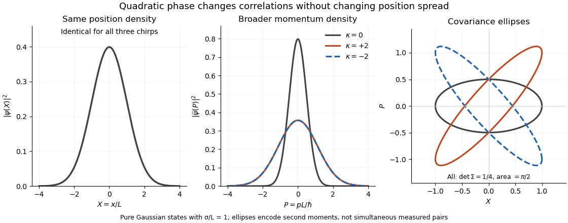
Quadratic phase preserves the position density but broadens the momentum density: opposite chirps tilt covariance ellipses in opposite directions while preserving their area
. Details. 
The phase space curves in the figure satisfy in the dimensionless coordinates, where . They display second moments, not observed simultaneous position and momentum pairs. Their common area is , although their coordinate projections differ.
This distinction is useful for predicting focusing. Under free particle evolution with mass , , soA negative chirp initially narrows the position distribution; positive chirp initially broadens it. For , the minimum occurs at and has variance . At that time the quantum covariance vanishes, and the unchanged momentum spread gives . The extra initial product was a usable position-momentum correlation, not extra measurement backaction.
Heisenberg's microscope Created 2026-10-18 Updated 2026-10-20
Heisenberg's microscope is a thought experiment, not a report of a performed measurement. In Werner Heisenberg's Nobel lecture, The development of quantum mechanics, delivered on 11 December 1933, the imagined electron is illuminated with very short-wavelength light and observed through a high-resolution microscope. A scattered photon entering the observer's eye would, through Compton scattering, eject the electron from its original path. The passage challenges a classical trajectory picture; its microscope is hypothetical. The lecture date is 1933 even though the award is the Nobel Prize in Physics in 1932.[ref]
The Development of Quantum Mechanics by Werner Heisenberg. Nobel Lectures, Physics 1922–1941; Werner Heisenberg, The development of quantum mechanics, heading and printed pp. 291–292; text inspected in the Studyres transcription
The following idealized geometry makes the tradeoff visible. Let the collected light have wavelength and let the microscope objective accept outgoing directions within a half-angle about the vertical axis. Take transverse to that axis and hold the incoming photon momentum fixed. A diffraction-limited estimate of transverse resolution has scale . The unobserved outgoing direction admits transverse photon momentum components between approximately and , neglecting the angular variation of the scattered wavelength. By conservation of momentum, uncertainty in that component leaves uncertainty in the transverse recoil of the electron:Here is the Planck constant; the two symbols denote heuristic resolution and recoil scales, not the standard deviations in the Heisenberg uncertainty relation. Increasing the acceptance angle improves the estimated resolution while broadening the allowed recoil range. Numerical factors depend on the resolution criterion and angular distribution; this scaling argument cannot supply the sharp constant .
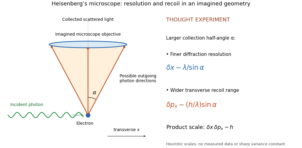
Heisenberg microscope thought experiment: an imagined scattering event and collection cone, with resolution and recoil scales rather than measured data
. Details. 
The thought experiment makes the interaction needed to obtain an image memorable. The preparation uncertainty theorem has broader use: it applies to the prepared quantum state even when the two observables are measured on separate copies. No claim that Werner Heisenberg built this gamma ray apparatus is needed to understand either argument.
There are unlisted articles, also show them or only show them.