
Preparation uncertainty 2026-10-18
Preparation uncertainty describes the outcome spread intrinsic to a specified quantum state preparation. Operationally, prepare many copies of the same quantum state, measure position on one group and momentum on another, and estimate the two variances. Ideal measurements still have the spreads predicted by the Born rule. No earlier position measurement need occur in the momentum group. The Heisenberg uncertainty relation constrains these two distributions belonging to the same preparation.
Measurement backaction concerns how a particular measurement in quantum mechanics changes a quantum state. Instrument resolution concerns how its reported outcomes relate to the intended observable. Those questions require a model of the instrument and its interaction with the system. Substituting an instrument error and an induced change for and in the Heisenberg uncertainty relation does not follow from its proof. The practical value of preparation uncertainty is that it bounds achievable input spreads before any such instrument model is chosen.
Confinement energy bound from position support Created 2026-10-18 Updated 2026-11-05
Suppose each Cartesian coordinate of a particle of mass is supported in an interval of length , in dimensions. Popoviciu's inequality on variances gives , and the Heisenberg uncertainty relation gives . Since ,This is a rigorous but non-sharp confinement estimate. For a cubical infinite square well, separation of variables gives the stronger exact ground-state value . One must not identify a support length with a uniquely prescribed standard deviation or claim that the uncertainty estimate is the exact ground-state energy.
Indoor-temperature limit of a Carnot heat pump Created 2026-10-18 Updated 2026-11-05
A reversible heat pump maintaining against an external has heating coefficient of performance . If its maximum work input is and the building loses heat at rate , maintaining equilibrium requires . This yields the displayed minimum external temperature, provided it lies in the physical positive-temperature range. If the rating instead specifies maximum delivered heat, the bound is ; a heat-output rating cannot be substituted for a work-input rating in the Carnot formula.
Optical trap calibration uncertainty 2026-10-18
Write for the detector's position-related voltage variance, after characterizing independent detector noise and the acquisition response. The equipartition theorem estimate is . For small independent input standard uncertainties, first-order propagation givesIn this expression is the uncertainty of the variance itself. If the assumed independent relative uncertainties are , , and , respectively, the resulting relative standard uncertainty is . This invented budget excludes model bias. Shared calibration inputs introduce covariance terms: a force estimate using this same thermal estimate has , so treating and as independent would count their sensitivity incorrectly.
Correlated Brownian motion also makes sample count a poor proxy for independent information. For a long continuous stationary Gaussian record of duration , estimating from gives, to leading order,The Gaussian distribution fourth-moment identity gives ; integrating this covariance over the observation interval gives the result. Subtracting a fitted mean changes higher-order terms when . The ideal example gives about relative uncertainty in the variance, even though samples were recorded. This ideal statistical estimate does not include drift, detector noise or incorrect drag.
Optical trap drag calibration Created 2026-10-18 Updated 2026-10-20
Translate the liquid past a bead held in a stationary harmonic optical trap. At steady mean position, take as the local fluid velocity relative to the fixed trap and positive downstream. Averaging the overdamped force balance givesFor the invented optical trap Langevin calibration example, predicts , , and . Reversing reverses the mean shift but leaves the ideal thermal variance unchanged. A symmetric speed sweep tests the offset and the linear force range; the slope determines if position is calibrated.
Near a wall, is not the appropriate drag without a boundary correction; record bead height and direction of motion. Stage velocity must correspond to the local fluid velocity after transients have settled. Escape under increasing flow estimates a maximum holding force in that geometry, whereas small-displacement drag calibration estimates the local spring constant. They are different quantities. The atomic force microscopy similarly needs a calibrated spring constant to convert a measured deflection to force, but its cantilever is a physical spring rather than this optical field.
Nondegenerate stationary points of a planar harmonic function Created 2026-10-18 Updated 2026-10-20
For a planar harmonic function, . Its Hessian matrix is therefore , with eigenvalues . At a stationary point with nonzero Hessian matrix determinant, both signs occur, so the point is a saddle point. A zero determinant requires separate treatment and is not covered by this nondegenerate test. The result is the local quadratic counterpart of the maximum principle for harmonic functions.
For bounded piecewise continuous Dirichlet boundary data on a circle of radius , write its Fourier series as . The displayed series gives the bounded exterior harmonic extension for . The radial inversion in a circle converts it into the ordinary interior Poisson kernel solution. Values at discontinuities are understood through the usual boundary trace, with midpoint radial limits at jumps; changing the assigned values at finitely many boundary points does not change the extension.
The limit at infinity is forced to equal the angular mean . Indeed the angular mean of any exterior harmonic function solves , and boundedness excludes its logarithmic term. Equivalently, inversion makes infinity an isolated removable singularity of a bounded planar harmonic function. Uniqueness follows from interior uniqueness after inversion, including the logarithmic cutoff proof of harmonic uniqueness with finitely many boundary exceptions when needed.
Hard-sphere S-wave scattering 2026-10-18
For a hard sphere of radius , the exterior radial S wave is proportional to . Matching it to gives scattering phase shift modulo and scattering length . The scattering amplitude is , giving the displayed cross section. The zero-energy limit is , its zeros occur at positive integer multiples , and its high-energy envelope decreases as . This is one partial wave, not the total high-energy hard-sphere result obtained by summing all partial waves.
Work by Hans Adolf Krebs 2026-10-18
Stellar intensity interferometry 2026-10-18
Stellar intensity interferometry measures a star's angular diameter by comparing fluctuations of detected light intensity at separated collectors. Each collector has its own photodetector; an analog multiplier or a digital correlator compares the electrical outputs. Changing the interferometric baseline changes the sampled spatial optical coherence. An unresolved star produces correlated fluctuations; a resolved extended source supplies different mixtures of emission directions, reducing their correlation.
This makes a useful telescope out of a surprising observable: the fluctuations discarded by an ordinary average-brightness measurement. Optical beams need not travel to a common combiner. A relative wave phase perturbation leaves unchanged, so pure phase errors do not directly change the local light intensity. Electronic delay alignment remains necessary; intensity changes from atmospheric scintillation, collection losses, and instrumental noise still require controls.
Let join the collectors and let be the unit line of sight toward the star. The relevant interferometric baseline is its projection onto the plane of the sky:The reference arrival-time difference has magnitude , with speed of light . Correct that delay, with a sign fixed by channel order, before averaging the residual correlation at . The physical collector separation equals only when it is perpendicular to ; tracking a star can change the projection even for fixed collectors.
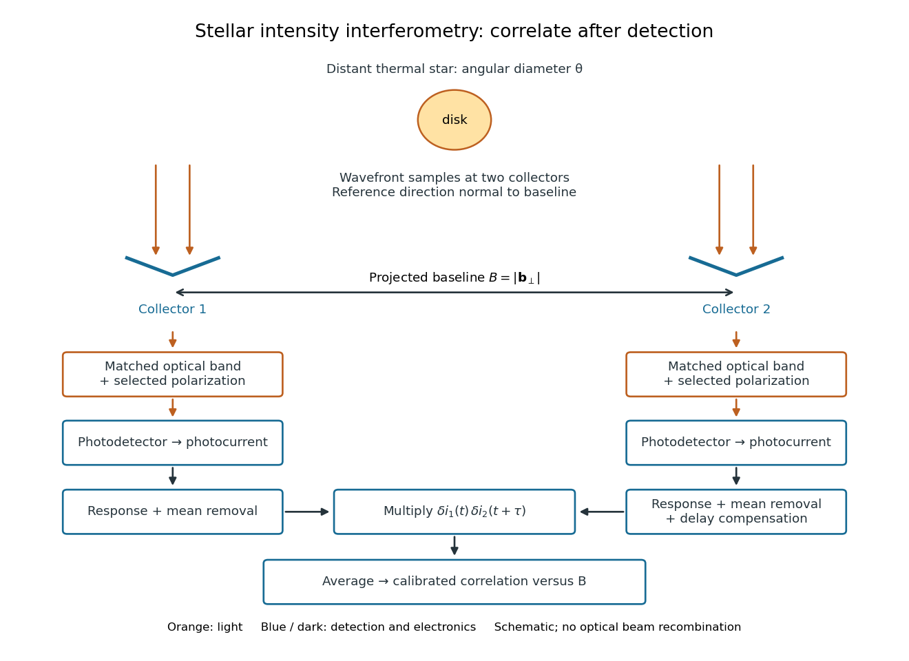
Functional geometry of stellar intensity interferometry: separate optical detection followed by electrical correlation
. Original schematic with the reference direction normal to the baseline. Matched optical selection feeds independent detectors; mean removal, response and delay alignment precede multiplication and averaging. This is not a scale drawing of the historical apparatus. Details.
Hénon-Heiles system 2026-10-18
The Hénon-Heiles system is a Hamiltonian system with two degrees of freedom and Hamiltonian functionIts Hamilton's equations give and . Its potential energy combines an isotropic quadratic minimum with a cubic interaction.
Removal of a half-oscillator wall Created 2026-10-18 Updated 2026-11-05
Suddenly remove the wall of a half-harmonic oscillator in its ground state, leaving the same harmonic potential on the whole line. The sudden approximation keeps its wavefunction unchanged during removal. The new normalized ground state is , soThe integration is over the initially occupied half-line. The final first excited state instead has probability , since the initial half-line state equals times its positive-half restriction. This also checks that removing the wall does not simply create the full oscillator's odd state.
Exponential trial state for a half-harmonic oscillator Created 2026-10-18 Updated 2026-11-05
For the dimensionless half-harmonic oscillator on with , the trial family , , is admissible for the Rayleigh-Ritz variational principle. The moments give norm squared , derivative energy , and potential energy . Its Rayleigh quotient is , minimized at . The resulting upper bound exceeds the exact lowest eigenvalue three; the exact ground-state shape is .
Inferring a binary from a detector network 2026-10-18
For detector , model the calibrated data as , with a shared source parameter vector , separate detector responses, propagation delays and noise . Under an independent stationary Gaussian process approximation with one-sided power spectral density , define the noise-weighted inner product and likelihood functionStrain power spectral density has units ; the displayed inner product is dimensionless when the Fourier transform integrates over seconds. A matched filter rewards agreement over the full evolving wave phase, weighting frequency bands by their noise. One conspicuous peak is insufficient: a candidate should also have the right distribution of signal across frequency bands and compatible projections in the network.
The parameter paper used coherent Bayesian inference, numerical relativity-informed inspiral–merger–ringdown models and explicit calibration uncertainties. It found a strong distance–inclination correlation; source-frame masses additionally require converting the detector-frame masses by a cosmological redshift.[ref]
Properties of the Binary Black Hole Merger GW150914 by B. P. Abbott and others. II Parameter estimation, equations (1)–(5), II.A waveform models; III Results, p. 7, Fig. 2
Conceptually, multiply the likelihood function by a prior distribution to obtain a posterior distribution. Changes in waveform families, residual structure after subtraction, and checks with a generic transient reconstruction test parts of the modeling assumptions. Detection significance and parameter uncertainty answer different questions. Coincidence and noise controls for GW150914 2026-10-18
The modeled matched filter search found an arrival difference of about , within the roughly intersite light travel time. Background events were obtained by shifting one detector's timestamps far beyond that time and repeating the coincidence analysis. The binary search bounded the false alarm rate below one event per years. That is an empirically estimated background rate, not a probability that the source interpretation is false.[ref]
The logic is to destroy a common astronomical arrival while retaining each instrument's real glitches. A Poisson distribution approximation would turn a background rate into for at least one equally strong noise event during live time , only after accounting for the search's ranking and trials. Repeated time slides reuse data; their accumulated background duration is not an equally long series of independent new observations. Correlated disturbances also require separate controls because shifting timestamps can erase them along with a true signal.
The dedicated noise study inspected auxiliary channels and deliberately applied magnetic, acoustic and mechanical disturbances to measure their coupling into strain. For GW150914, checks included environmental coincidences, instrument state, and exclusion of an intentional hardware injection. It also examined potentially correlated global magnetic disturbances, which time slides alone cannot exclude.[ref]
Characterization of transient noise in Advanced LIGO relevant to gravitational wave signal GW150914 by B. P. Abbott and others. 2 Identifying noise sources, Fig. 2; 6 Validation of GW150914; Appendix B physical environment monitors
The point of an injection test is quantitative: a quiet environmental monitor is informative only if its sensitivity and coupling bound the disturbance needed to explain the candidate. LIGO differential strain measurement 2026-10-18
Each LIGO instrument is a Michelson interferometer with approximately arms containing Fabry–Pérot interferometers. A stabilized laser illuminates suspended fused-silica mirrors in vacuum. Four-stage suspensions and active isolation suppress ground motion; low-loss materials reduce thermal noise. Power recycling increases circulating power; signal recycling shapes the response to the gravitational wave.[ref]
Why measure two perpendicular arms? In the long-wavelength limit, take a gravitational wave with plus polarization normally incident on ideal perpendicular arms. Its transverse-traceless tensor has and . Expanding each proper length to first order givesHere is dimensionless, whereas is a length. A stipulated and imply , with individual arm changes of opposite sign and magnitude . These are equivalent differential arm-length changes, not a photograph of mirrors moving against a rigid external ruler. The observable compares returning light phases; coordinate systems can distribute the description between mirror coordinates and light propagation.
For unit arm directions , define the detector tensor . If are the transverse polarization tensors, thenThe dimensionless factors encode sky direction and the polarization basis. Thus even identical sources can have different observed amplitudes and wave phases. Motion changing both arms equally cancels in this ideal differential observable, although real asymmetries can couple common disturbances into it.
Suspension supplies an inertial reference above its resonances. For example, a single ideal harmonic oscillator with support motion obeys . Its response at angular frequency is , which decreases in magnitude as well above resonance. The mirror follows slow support drift but approximately free motion in the high-frequency limit. Real multistage suspensions also require damping and alignment control; resonant frequencies are not regions of good isolation.
Rainer Weiss's 1972 report proposed suspended masses, multiple-pass optical delay lines, and a servo holding an interference fringe. Its noise analysis separately treats photon-counting fluctuations, laser frequency instability, mechanical thermal noise, radiation pressure and ground motion. Those delay lines should be distinguished from the resonant arm cavities of Advanced LIGO.[ref]
Electromagnetically coupled broadband gravitational antenna by Rainer Weiss. Typeset transcription of 1972 report, sections 4–5.5, Fig. 1; original scan is linked from DCC record P720002
Work by Gustaf Dalén 2026-10-18
Work by Günter Blobel 2026-10-18
One-dimensional representation 2026-10-18
A one-dimensional complex group representation acts on a one-dimensional complex vector space, and is equivalently a group homomorphism into the multiplicative group . It is automatically an irreducible representation. Its character of a representation is its scalar value, a one-dimensional character. A change of basis cannot change those scalar values, so two such group representations are equivalent exactly when their homomorphisms agree. For a symmetric group with , all transpositions are conjugate, square to the identity and generate the group. Their common scalar image is therefore or , giving exactly the trivial representation and the sign representation.
Inverse-adjoint representation Created 2026-10-18 Updated 2026-11-05
For a complex finite-dimensional group representation, the displayed matrices give another group representation: taking inverses and taking the conjugate transpose each reverse multiplication order, so their composition preserves it. This operation is involutive. With the standard Hermitian inner product, an invariant vector subspace for has orthogonal complement invariant for , because . Thus for . It follows that is an irreducible representation exactly when is. No finiteness assumption on the group or unitarity assumption on the group representation is needed.
There are unlisted articles, also show them or only show them.