
Gaussian covariance in a harmonic potential 2026-10-18
Under a quantum harmonic oscillator Hamiltonian, the Heisenberg equations of motion giveSubtract the expectation values, square the first equation, and use the symmetrized covariance . This yieldsThese moment equations hold for any state with finite second moments; a quadratic Hamiltonian additionally preserves Gaussian wave packets. A coherent state has , , and , so its width stays fixed while its center follows the classical orbit. A squeezed coherent state generally has a width that oscillates at .
Gaussian trial for a quadratic-plus-quartic oscillator Created 2026-10-18 Updated 2026-11-05
For , use the normalized real wavefunction , . The Gaussian integral gives and , while the kinetic contribution is . Thus the Rayleigh quotient is the displayed expression. For positive , its stationary width satisfies . At the unique positive solution is , giving by the Rayleigh-Ritz variational principle. For , taking makes the negative quartic contribution dominate, so the energy is unbounded below even within this normalized family. The positive-coupling bound and negative-coupling instability concern different signs of the same variational expression.
Near-axis radial magnetic field Created 2026-10-18 Updated 2026-10-20
For a smooth axisymmetric magnetic field, write . The absence of magnetic monopoles gives . Integrating from the axis and excluding a singular term proves the displayed relation. An axial field decreasing along has an outward radial component, even when the field points purely axially on the axis itself.
Lattice gauge theory Created 2026-10-18 Updated 2026-11-05
A formulation of a gauge theory with discretized spacetime. Matter fields are assigned to sites and gauge-group elements to links between nearby sites. Products of link variables around closed paths provide gauge-invariant quantities. This structure preserves the local gauge symmetry while making nonperturbative numerical calculations possible. Physical predictions require control of finite spacing, finite volume and statistical errors rather than treating one finite grid as the continuum theory.
Gas-discharge lamp 2026-10-18
Thyratron Created 2026-10-18 Updated 2026-11-05
A thyratron is a gas-filled electronic switching tube in which a control electrode triggers a conducting discharge between cathode and anode. The control signal governs the onset of conduction, allowing a comparatively small trigger to switch a larger supplied pulse of electric current.
Once the discharge is established, the control electrode does not act like a continuously adjustable linear gain control. The external circuit must bring the current down sufficiently for the gas to recover its nonconducting state. Trigger timing, recovery and the load circuit therefore determine repeated-pulse behavior. This distinguishes a thyratron switch from a linear electronic amplifier.
Gas-globe density measurement 2026-10-18
In an idealized rigid-globe weighing, subtract the evacuated assembly's mass from the filled assembly's mass, then divide by the internal volume. Establish the filled sample's pressure and temperature before comparing gases. The subtraction removes the container's large contribution, making a small gas contribution accessible. A real measurement also needs corrections or bounds for residual gas, adsorption, leaks, changing vessel volume and external buoyancy. The Rayleigh-Ramsay argon density experiment shows why preparation-route comparisons add information beyond repeated weighings of one sample.
Electric quadrupole transition Created 2026-10-18 Updated 2026-10-25
An electric quadrupole transition is a radiative transition of an atomic nucleus with electric multipole order two. The emitted photon carries two units of angular momentum and positive parity, so the atomic nucleus has unchanged parity.[ref]
NuDat 3 Glossary by National Nuclear Data Center. Multipolarity, E2 entry
Addition of angular momentum imposes . Thus and can be E2, whereas cannot emit one E2 photon. On the even-, nuclear rotational band, the adjacent downward transitions have ; that band pattern is more restrictive than the general E2 selection rule.
Work by G. R. Williams 2026-10-18
Implicit function 2026-10-18
An implicit function is a function specified through a relation between its input and output, rather than an explicit output formula. Locally, an equation may specify if one output is selected for each input in a suitable domain. Different branches can define different functions; the relation itself need not give a unique output globally. For example, gives the two branches on .
The implicit function theorem gives sufficient conditions for a unique local differentiable branch, while implicit differentiation computes its derivative by the chain rule. If is continuously differentiable and , that derivative is along the branch.
Scalar-valued function Created 2026-10-18 Updated 2026-10-20
A scalar-valued function is a function whose codomain is a field, typically the real numbers or complex numbers. Its output is a single scalar, while its input can belong to an arbitrary set. For example, the square of the norm of a vector is real-valued. In a relativistic application, being scalar-valued alone does not establish Lorentz invariance: the transformation of the input and of the complete quantity must also be specified.
Optical normalization of Fresnel integrals 2026-10-18
For the optical convention of Fresnel integrals, and . Both functions are odd and tend to as . If the unscaled convention uses phase , multiply its argument by and its value by to obtain this convention. An aperture factor with phase uses . Stating the convention prevents missing factors of or in diffraction calculations.
Near-field diffraction laboratory experiment 2026-10-18
A documented experiment uses curved illumination rather than the uniform Fresnel slit propagation model. Laboratory Exercise No. 4: Diffraction, MIT 6.237, Fall 2024, printed pp. 5–6, gives a helium–neon laser at , a microscope objective optical lens, a circular aperture and a screen 5–40 cm from the object. Preparation includes comparing central brightness in Fresnel diffraction and Fraunhofer diffraction. A 40× objective produces a nonplanar incident wavefront; the opening is placed less than 1 cm from it. With objective-to-screen distance fixed, students move the opening, sketch patterns, and record positions of consecutive central nulls to estimate aperture size. The Fraunhofer diffraction pattern supplies a regime comparison. A separate spherical-obstacle task observes a bright centre inside the shadow. The handout supplies procedures, rather than measured distances or profiles.[ref]
The circular-opening test probes cancellation of complex amplitudes at the centre while the source wavefront curvature changes. To interpret it, include that curvature in the aperture field and use a circular aperture, rather than substituting the plane-illuminated Fresnel slit propagation profile. Useful additional controls are to retain the same laser and opening, centre the illumination, repeat position readings and check background with the beam blocked. If a camera replaces the visual screen readout, avoid saturation and calibrate its position scale. Alignment, imperfect aperture edges, illumination variation and limited contrast near a null constrain the inferred size. A bright central obstacle spot illustrates why the sharp shadows of geometrical optics can fail; it does not imply that every Fresnel diffraction pattern has a bright centre.
Fresnel slit propagation 2026-10-18
Consider a uniform plane wave of unit complex amplitude transmitted by an ideal optical slit of full width . Treat the field as invariant along the optical slit height: this is one-dimensional transverse Fresnel propagation, so the prefactor is , rather than the two-dimensional prefactor . Removing the carrier givesHere is incident irradiance. This infinitely long slit model describes a transverse cut away from the ends of a sufficiently long physical slit; its finite conserved quantity is transmitted power per unit optical slit height.
Put and . Substitution reduces the integral toThis form separates the pattern's shape from its physical scale. Reflection proves , so the light intensity is an even function of . At , direct integration gives , with limit one at . Hence the Fraunhofer diffraction comparison is the squared sinc function. In this paragraph the unnormalized sinc function takes argument .
For an original example, choose wavelength and full width . At , , and the edge-to-centre wave phase change is radians. At , , and that wave phase change is only radians. Even the nearer screen is fifty slit widths away; that geometric comparison alone misses its strong Fresnel diffraction.
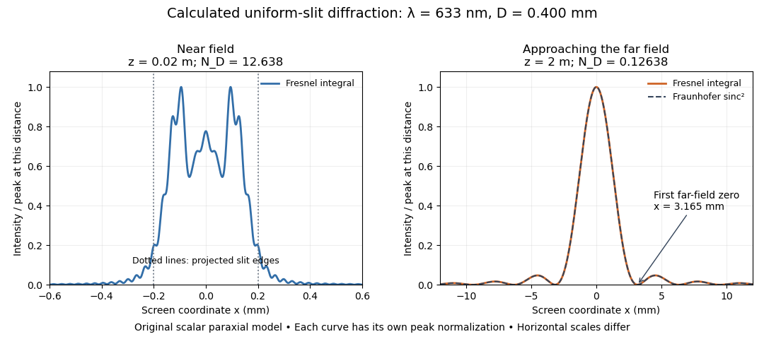
Original calculated Fresnel diffraction profiles of a 0.400 mm slit at 633 nm, compared with the Fraunhofer diffraction shape
. Details. 
These are numerical predictions from the displayed scalar integral, using the composite trapezoidal rule, rather than measured profiles. Each curve is divided by its own peak light intensity; the two horizontal scales differ. At 2 cm the computed central irradiance is about , with brighter off-axis maxima. At 2 m it is about and is the peak. The dashed Fraunhofer diffraction curve has its own central normalization; its first zeros are at . The finite-distance Fresnel diffraction curve remains slightly nonzero there.
Normalization hides the brightness change, but not the change in shape. The Fourier transform propagation multiplier has unit complex modulus, so Plancherel theorem givesThis is conservation of transmitted power per unit height in the ideal scalar model. An integral over only the displayed screen interval misses the tails; a peak-normalized profile is not a unit-integral probability density. Spreading and decreasing brightness together preserve the transmitted power.
Fresnel number 2026-10-18
A Fresnel number compares squared aperture size with the product of wavelength and propagation distance. For an optical slit of full width , explicitly distinguish the full-width and half-width conventions:The full-width convention is used throughout the Fresnel slit propagation example below. The definition also appears in the Delft treatment.[ref]
Scalar Diffraction Optics. Interactive Optics by Sander Konijnenberg, Aurèle J.L. Adam and H. Paul Urbach; Fresnel and Fraunhofer Approximations, equations (390)–(392): aperture diameter convention
For uniform incident wave phase, makes the omitted aperture wave phase small and gives the Fraunhofer diffraction regime. When is of order one or larger, retain it and use Fresnel diffraction, provided the paraxial approximation still holds. These are continuous changes in accuracy, rather than a physical boundary at one selected number. For a rectangular aperture, check both transverse dimensions. Incident wavefront curvature contributes its own wave phase through ; the aperture-to-screen Fresnel number alone does not describe a spherical source's illumination.
The scaling is revealing: doubling the optical slit width at fixed wavelength and distance multiplies the Fresnel number by four. Maintaining the same Fresnel number then requires four times the distance. Two systems can consequently have the same dimensionless pattern despite very different physical lengths.
Fresnel diffraction phase curvature 2026-10-18
The quadratic wave phase follows from an ordinary distance calculation. Write . The Taylor expansion of the distance to a screen point isIn the slowly varying propagation prefactor, suffices. In the complex exponential , however, a small distance error is multiplied by the large wavenumber . Retaining the quadratic term while dropping the quartic term requires both and over the contributing aperture and the screen region being considered. The second condition is a wave phase accuracy requirement; the first is the geometric paraxial approximation.
Expanding the retained quadratic term separates three effects:The outside quadratic factor changes the wave phase at each screen point but has unit complex modulus, so it leaves that screen's light intensity unchanged. The quadratic factor inside the integral changes relative wave phases between contributions from different aperture points, so it changes their wave interference. The remaining linear factor supplies a Fourier transform. Fraunhofer diffraction drops the aperture quadratic factor when it is nearly constant; it does not require dropping the screen quadratic factor when predicting a later coherent field.
There is also a useful proof from the Helmholtz equation. Substituting gives . Neglecting yields the parabolic wave equation. A transverse Fourier transform evolves each spatial frequency by , using the transform kernel . Its inverse Fourier transform is the quadratic Fresnel propagator kernel above. Thus quadratic wave phase in space and quadratic wave phase in spatial frequency are two views of the same propagation.
Square-aperture Fresnel diffraction 2026-10-18
For an axial point source a distance before a square aperture and an observer a distance beyond it, source and observation wave phase curvatures add: . With aperture side , put . Separation into two one-dimensional Fresnel integrals gives the field normalized to its unobscured value,At an off-axis observer , centre the dimensionless coordinates on and . If are the directed Cornu spiral chords between the corresponding aperture-edge parameters, . This is a product of complex interval factors, rather than a sum of two intensities. The unobscured field is evaluated at the same observation point and includes its common propagation wave phase.
Fresnel half-period zone 2026-10-18
A Fresnel half-period zone is a region of an aperture whose optical path to an observation point differs from the axial path by an interval of half a wavelength. For an axial optical point source a distance before the aperture and an axial observer a distance beyond it, the paraxial path excess at aperture radius is . The outer radius of zone is thereforeSuccessive zones contribute approximately opposite phases to the Huygens-Fresnel principle integral. The finite source distance matters: using the plane-wave formula requires .
Fresnel diffraction by a circular aperture 2026-10-18
For a circular aperture of radius , paraxial plane-wave illumination and propagation distance , define . On axis, the radial Fresnel diffraction integral normalized by the unobstructed field givesFor a finite axial point source a distance before the aperture and detector a distance after it, replace by in the phase. The formula assumes illumination amplitudes and obliquity factors approximately constant across the aperture. Odd and even numbers of Fresnel half-period zones give bright and dark axial extrema; large local intensity is compatible with global conservation of energy.
Fresnel diffraction by an opaque disk 2026-10-18
Under the same scalar paraxial assumptions as Fresnel diffraction by a circular aperture, Babinet's principle gives the complementary opaque-disk field on axis. Its axial intensity equals the unobstructed intensity, producing the Arago spot inside the geometric shadow. The off-axis pattern depends on the full Fresnel integral; it is not obtained by subtracting aperture intensities from the incident intensity. Finite source size, misalignment and imperfect circular edges reduce the ideal spot contrast.
There are unlisted articles, also show them or only show them.